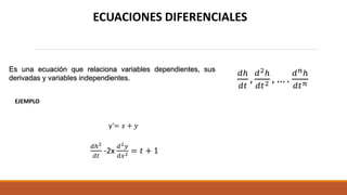
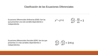
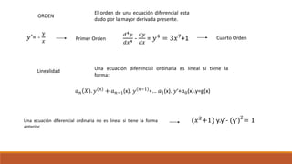
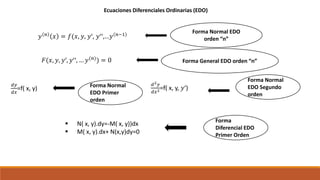
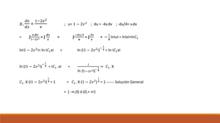
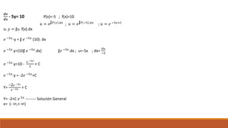
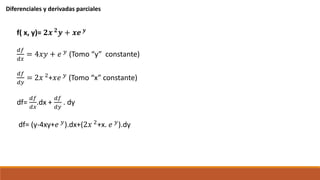
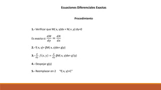
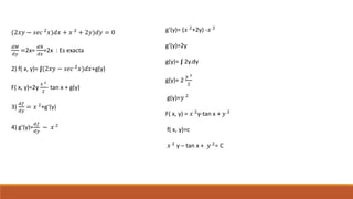
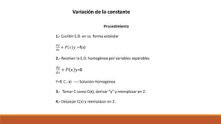
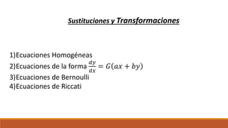
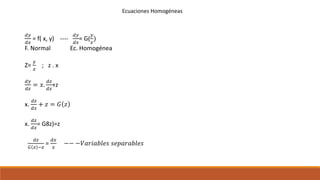
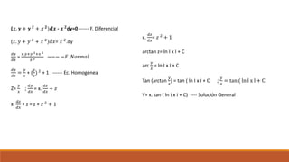
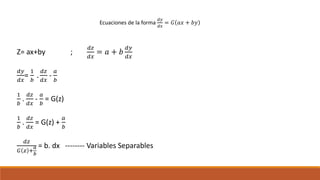
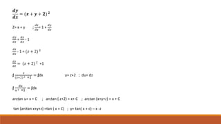
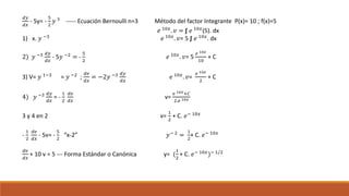
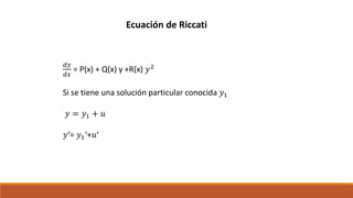
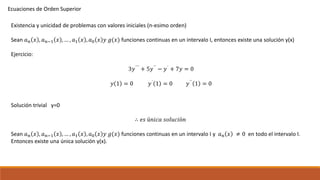
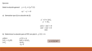
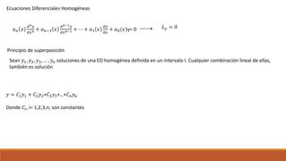
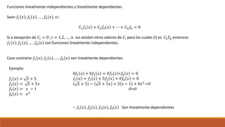
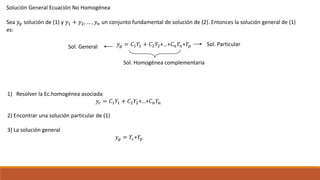
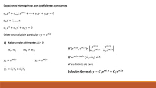
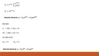
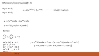
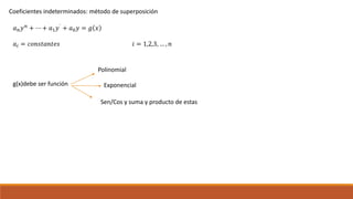
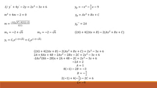
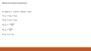
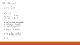
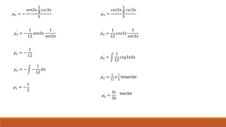
UNIVERSIDAD POLITÉCNICA SALESIANA
TRABAJO REMEDIAL DE MATEMÁTICAS
NOMBRE: DENNISSE VANESSA LEONES AGUA
GRUPO 1
Es una ecuación que relaciona variables dependientes, sus
derivadas y variables independientes.
𝑑ℎ
𝑑𝑡
,
𝑑2ℎ
𝑑𝑡2 , … .
𝑑 𝑛ℎ
𝑑𝑡 𝑛
𝑑ℎ2
𝑑𝑡
-2x
𝑑2 𝑦
𝑑𝑥2 = 𝑡 + 1
y‘= 𝑥 + 𝑦
ECUACIONES DIFERENCIALES
EJEMPLO
Clasificación de las Ecuaciones Diferenciales
Ecuaciones Diferenciales Ordinarias (EDO): Son las
que presentan una sola variable dependiente e
independiente.
Ecuaciones Diferenciales Parciales (EDP): Son las que
presentan 2 o más variables dependientes e
independientes.
𝑑2 𝑦
𝑑𝑥2 -
𝑑𝑦
𝑑𝑥
= 1𝑦‘‘−𝑦‘=1
𝑑2 𝑥
𝑑𝑦2 -
𝑑2 𝑧
𝑑𝑡2 = 1+t-y
ORDEN
El orden de una ecuación diferencial esta
dado por la mayor derivada presente.
𝑑4 𝑦
𝑑𝑥4 -
𝑑𝑦
𝑑𝑥
= 𝑦4 = 3𝑥7+1𝑦‘= -
𝑦
𝑥
Primer Orden Cuarto Orden
Linealidad Una ecuación diferencial ordinaria es lineal si tiene la
forma:
𝑎 𝑛 𝑋 . 𝑦(𝑛) + 𝑎 𝑛−1(x). 𝑦(𝑛−1)+... 𝑎1(x). 𝑦‘+𝑎0(x).y=g(x)
Una ecuación diferencial ordinaria no es lineal si tiene la forma
anterior.
(𝑥2
+1) y.y‘- (y‘)2
= 1
Campos Direccionales
Implícita: f(y‘,y,x)=0
Ejemplo:
Explícita: y‘(x)=f(y(x),x)
Ejemplo:
y‘-x-y=0y‘=x+y
Solución de una Ecuación Diferencial:
Una función y=d(x) es una solución de una E.D.O. de
orden “n” en un intervalo I, si sus “n” derivadas existen
en el intervalo I y al reemplazarlas en las E.D. se
obtiene una identidad.
𝒚 =
𝟏
𝒙
𝑦‘= −
1
𝑥2
𝑦‘‘=
1
𝑥3
𝑦‘‘= 𝑦3
𝒚‘ =
𝟏
𝒙
𝒆𝒔 𝒔𝒐𝒍𝒖𝒄𝒊ó𝒏 𝒅𝒆𝑦‘‘= 𝑦3
en (- ∞,0) o (0+ ∞)
X=(- ∞,0) u (0+ ∞)
X=(- ∞,0) u (0+ ∞)
Ecuaciones Diferenciales Ordinarias (EDO)
𝐹(𝑥, 𝑦, 𝑦‘, 𝑦‘‘, … 𝑦(𝑛)) = 0 Forma General EDO orden “n”
𝑦 𝑛
𝑥 = 𝑓(𝑥, 𝑦, 𝑦‘, 𝑦‘‘,…𝑦 𝑛−1
Forma Normal EDO
orden “n”
𝑑𝑦
𝑑𝑥
=f( x, y) Forma Normal
EDO Primer
orden
𝑑2 𝑦
𝑑𝑥2=f( x, y, 𝑦‘)
Forma Normal
EDO Segundo
orden
 N( x, y).dy=-M( x, y))dx
 M( x, y).dx+ N(x,y)dy=0
Forma
Diferencial EDO
Primer Orden
Problemas con Valores Iniciales (PVI)
Consiste en encontrar una solución particular y (x) que cumple ciertas condiciones dadas:
𝑅𝑒𝑠𝑜𝑙𝑣𝑒𝑟:
𝑑 𝑛 𝑦
𝑑𝑥 𝑛 = 𝐹(𝑥, 𝑦, 𝑦‘,𝑦‘‘, … 𝑦 𝑛−1 )
Sujeto a:
𝑦(𝑥0) = 𝑦0, 𝑦‘(𝑥0) = 𝑦1,𝑦‘‘(𝑥0) = 𝑦2, … 𝑦 𝑛−1
(𝑥0) = 𝑦 𝑛−1
Procedimiento:
1.- Encontrar la solución n- paramétrica.
2.- Usar los valores iniciales para hallar los “n” parámetros.
3.- Escribir la solución particular.
Ejemplo:
X(o)=300 ; x‘(0)=0
X=(0) t +
𝟏
𝟐
(-9,8) 𝑡2+300 ----- Solución Particular
X(5)=
𝟏
𝟐
(-9,8). (5)2
+300
F= m . g ; x(0)=300
a=g ; x‘(0)=0
𝑑2 𝑥
𝑑𝑡2 = g ;
𝑑𝑥
𝑑𝑡
= g.t+𝐶1
X=
𝟏
𝟐
. g . 𝑡2 + 𝐶1. t + 𝐶2 ----- Solución General
0=g(0) + 𝐶1
𝐶1=0
300=
𝟏
𝟐
. g. (0)2 + 𝐶1 (0) + 𝐶2
𝐶2= 300 ; (𝑉0)
X=
𝟏
𝟐
. g. 𝑡2
+ (0) t + 300
X =
𝟏
𝟐
g . 𝑡2 + 300 --- Solución Particular
X(5)=
𝟏
𝟐
(-9,8). (5)2 + 300
X(5)= 177,5 m.
Ecuaciones Diferenciales de Variables Separables
Dada la E.D.
𝒅𝒚
𝒅𝒙
= f x, y , si f x, y
Se puede separar en dos factores g(x) y h(y), entonces se habla de una E.D. de variables separables.
𝒅𝒚
𝒅𝒙
= 𝒇 𝒙, 𝒚 −−−− −
𝒅𝒚
𝒅𝒙
= 𝒈 𝒙 . 𝒉(𝒙)
(1+x) . dy - y . dx =0
(1+x) dy = y. dx
∫
𝒅𝒚
𝒚
= ∫
𝒅𝒙
(𝟏+𝒙)
lnIyI= ln(1+x) + 𝐶1
𝑒ln I 𝑦I= 𝑒ln (1+x)+ 𝐶1
IyI= 𝑒ln (1+x) . 𝑒 𝐶1
IyI= I1+xI . 𝐶2
Y=C (1+x) ----- Solución General
𝑥.
𝑑𝑣
𝑑𝑥
=
1−2𝑣2
𝑣
; u= 1 − 2𝑣2
; du = -4v.dv ; -du/4= v.dv
= ∫
𝒗.𝒅𝒗
1−2𝑣2 = ∫
𝒅𝒙
𝒙
= ∫
−du/4
𝒖
= ∫
dx
𝒙
= −
1
𝟒
lnIuI = lnIxI+ln𝐶1
lnI1 − 2𝑣2I= ln I𝐶1xI = ln (I1 − 2𝑣2I)
−
1
𝟒 = ln I𝐶1xI
ln (I1 − 2𝑣2I)
−
1
𝟒 = I𝐶1. xI =
1
ln (I1−2𝑣2I)
−
1
𝟒
= 𝐶1. X
𝐶1. X (I1 − 2𝑣2
I)
1
𝟒 = 1 = 𝐶1. X (1 − 2𝑣2
)
1
𝟒 = 1 ------ Solución General
= (- ∞,0) ó (0,+ ∞)
Método del Factor Integrante para EDO‘s (Lineales
Orden 1)
Procedimiento:
1.- Escribir la E.D. en su forma estándar.
𝑑𝑦
𝑑𝑥
+ 𝑃 𝑥 . 𝑦 = 𝑓 𝑥
2.- Encontrar el factor integrante 𝑢 = 𝑒∫ 𝑃 𝑥 .𝑑𝑥
3.- Escribir 𝑢. 𝑦 = ∫u. f(x).dx
4.- Resolver integral y despejar “y”.
𝒅𝒗
𝒅𝒙
- 5y= 10 P(x)=-5 ; f(x)=10
𝑢 = 𝑒∫ 𝑃 𝑥 .𝑑𝑥
; 𝑢 = 𝑒∫ 𝑃 −5 .𝑑𝑥
; 𝑢 = 𝑒 −5𝑥+𝐶
𝑢. 𝑦 = ∫u. f(x).dx
𝑒 −5𝑥
-y = ∫ 𝑒 −5𝑥
(10). dx
𝑒 −5𝑥.y=(10∫ 𝑒 −5𝑥.dx) ∫𝑒 −5𝑥.dx ; u=-5x ; dx=
𝑑𝑢
−5
𝑒 −5𝑥
.y=10 -
𝑒 −5𝑥
5
+ C
𝑒 −5𝑥
.y = -2𝑒 −5𝑥
+C
Y=
−2 𝑒 −5𝑥
𝑒 −5𝑥 + C
Y= -2+C 𝑒 5𝑥
-------- Solución General
x= (- ∞,+ ∞)
Diferenciales y derivadas parciales
f( x, y)= 𝟐𝒙 𝟐
𝒚 + 𝒙𝒆 𝒚
𝑑𝑓
𝑑𝑥
= 4𝑥𝑦 + 𝑒 𝑦 (Tomo “y” constante)
𝑑𝑓
𝑑𝑦
= 2𝑥 2+𝑥𝑒 𝑦 (Tomo “x” constante)
df=
𝑑𝑓
𝑑𝑥
.dx +
𝑑𝑓
𝑑𝑦
. dy
df= (y-4xy+𝑒 𝑦).dx+(2𝑥 2+x. 𝑒 𝑦).dy
Ecuaciones Diferenciales Exactas
En matemáticas, una ecuación
diferencial exacta es una ecuación
diferencial ordinaria de primer orden
que se presenta de la forma:
Una Ecuación Diferencial M( x, y).dy=0,
es exacta si existe una función f( x, y)=0,
tal que
𝑑𝑓
𝑑𝑦
=M(x , y) y
𝑑𝑓
𝑑𝑥
=N( x, y)
Criterio de Exactitud:
Una E.D. exacta cumple que:
𝒅𝑴
𝒅𝒚
=
𝒅𝑵
𝒅𝒙
Ecuaciones Diferenciales Exactas
Procedimiento
1.- Verificar que M( x, y)dx + N( x ,y) dy=0
Es exacta si:
𝑑𝑀
𝑑𝑦
=
𝑑𝑁
𝑑𝑥
2.- f( x, y)= ∫M( x, y)dx+ g(y)
3.-
𝑑
𝑑𝑦
𝑓 𝑥, 𝑦 =
𝑑
𝑑𝑦
∫M( x, y)dx+ g‘(y)
4.- Despejar g(y)
5.- Reemplazar en 2 “f( x, y)=C”
(2𝑥𝑦 − 𝑠𝑒𝑐 2 𝑥)𝑑𝑥 + 𝑥 2 + 2𝑦)𝑑𝑦 = 0
𝑑𝑀
𝑑𝑦
=2x=
𝑑𝑁
𝑑𝑥
=2x : Es exacta
2) f( x, y)= ∫(2𝑥𝑦 − 𝑠𝑒𝑐 2
𝑥)𝑑𝑥+g(y)
F( x, y)=2y
𝑥 2
2
- tan x + g(y)
3)
𝑑𝑓
𝑑𝑦
= 𝑥 2+g‘(y)
4) g‘(y)=
𝑑𝑓
𝑑𝑦
− 𝑥 2
g‘(y)= (𝑥 2+2y) -𝑥 2
g‘(y)=2y
g(y)= ∫ 2y.dy
g(y)= 2
𝑦 2
2
g(y)=𝑦 2
F( x, y) = 𝑥 2y-tan x + 𝑦 2
f( x, y)=c
𝑥 2
y – tan x + 𝑦 2
= C
Variación de la constante
Procedimiento
1.- Escribir E.D. en su forma estándar
𝑑𝑦
𝑑𝑥
+ 𝑃 𝑥 𝑦 =f(x)
2.- Resolver la E.D. homogénea por variables separables
𝑑𝑦
𝑑𝑥
+ 𝑃 𝑥 𝑦=0
Y=f( C , x) ---- Solución Homogénea
3.- Tomar C como C(x), derivar “y” y reemplazar en 2.
4.- Despejar C(x) y reemplazar en 2.
𝒅𝒚
𝒅𝒙
+y= 𝒆 𝟑𝒙
2) y= C. 𝑒 −𝑥
---- Solución Homogénea
𝑑𝑦
𝑑𝑥
+y=0 ----- Solución Homogénea
𝑑𝑦
𝑑𝑥
=
𝑑
𝑑𝑥
= (C. 𝑒 −𝑥
)
𝑑𝑦
𝑑𝑥
= - y
𝑑𝑦
𝑑𝑥
=
𝑑𝐶
𝑑𝑥
. 𝑒 −𝑥
+ 𝐶.
𝑑
𝑑𝑥
(𝑒 −𝑥
)
𝑑𝑦
𝑦
= −𝑑𝑥 3)
𝑑𝑦
𝑑𝑥
=
𝑑𝐶
𝑑𝑥
. 𝑒 −𝑥 - C. 𝑒 −𝑥 ---- 2 y 3 en 1
ln I y I= -x + 𝐶1 (
𝑑𝐶
𝑑𝑥
. 𝑒 −𝑥
- C 𝑒 −𝑥
) + C 𝑒 −𝑥
= 𝑒 3𝑥
𝑒 𝑙𝑛𝐼𝑦𝐼= 𝑒 −𝑥+𝐶1
𝑑𝐶
𝑑𝑥
. 𝑒 −𝑥=𝑒 3𝑥 ;
𝑑𝐶
𝑑𝑥
= 𝑒 4𝑥
I y I= 𝑒 𝐶1. 𝑒 −𝑥
4) C= ∫𝑒 4𝑥
.dx=
1
4
𝑒 4𝑥
+ 𝐶1 ---- 4 en 2
y= C. 𝑒 −𝑥
y=
1
4
. 𝑒 3𝑥
+ 𝐶1. 𝑒 −𝑥
Sustituciones y Transformaciones
1)Ecuaciones Homogéneas
2)Ecuaciones de la forma
𝑑𝑦
𝑑𝑥
= 𝐺 𝑎𝑥 + 𝑏𝑦
3)Ecuaciones de Bernoulli
4)Ecuaciones de Riccati
Ecuaciones Homogéneas
𝑑𝑦
𝑑𝑥
= f( x, y) ----
𝑑𝑦
𝑑𝑥
= G(
𝑦
𝑥
)
F. Normal Ec. Homogénea
Z=
𝑦
𝑥
; z . x
𝑑𝑦
𝑑𝑧
= 𝑥.
𝑑𝑧
𝑑𝑥
+z
x.
𝑑𝑧
𝑑𝑥
+ 𝑧 = 𝐺 𝑧
x.
𝑑𝑧
𝑑𝑥
= G8z)=z
𝑑𝑧
𝐺 𝑧 −𝑧
=
𝑑𝑥
𝑥
−− −𝑉𝑎𝑟𝑖𝑎𝑏𝑙𝑒𝑠 𝑠𝑒𝑝𝑎𝑟𝑎𝑏𝑙𝑒𝑠
(𝒙. 𝒚 + 𝒚 𝟐
+ 𝒙 𝟐
)𝒅𝒙 - 𝒙 𝟐
dy=0 ------ F. Diferencial
(𝑥. 𝑦 + 𝑦 2 + 𝑥 2)𝑑𝑥= 𝑥 2.dy
𝑑𝑦
𝑑𝑥
=
𝑥.𝑦+𝑦 2+𝑥 2
𝑥 2 −−− −𝐹. 𝑁𝑜𝑟𝑚𝑎𝑙
𝑑𝑦
𝑑𝑥
=
𝑦
𝑥
+ (
𝑦
𝑥
) 2
+ 1 ------ Ec. Homogénea
Z=
𝑦
𝑥
;
𝑑𝑦
𝑑𝑥
= x.
𝑑𝑧
𝑑𝑥
+ 𝑧
x.
𝑑𝑧
𝑑𝑥
+ z = z + 𝑧 2
+ 1
x.
𝑑𝑧
𝑑𝑥
= 𝑧 2
+ 1
arctan z= ln I x I + C
arc
𝑦
𝑥
= ln I x I + C
Tan (arctan
𝑦
𝑥
) = tan ( ln I x I + C ;
𝑦
𝑥
= tan ( ln l x l + C
Y= x. tan ( ln I x I + C) ---- Solución General
Ecuaciones de la forma
𝑑𝑦
𝑑𝑥
= 𝐺 𝑎𝑥 + 𝑏𝑦
Z= ax+by ;
𝑑𝑧
𝑑𝑥
= 𝑎 + 𝑏
𝑑𝑦
𝑑𝑥
𝑑𝑦
𝑑𝑥
=
1
𝑏
.
𝑑𝑧
𝑑𝑥
-
𝑎
𝑏
1
𝑏
.
𝑑𝑧
𝑑𝑥
-
𝑎
𝑏
= G(z)
1
𝑏
.
𝑑𝑧
𝑑𝑥
= G(z) +
𝑎
𝑏
𝑑𝑧
𝐺 𝑧 +
𝑎
𝑏
= b. dx -------- Variables Separables
𝒅𝒚
𝒅𝒙
= (𝒙 + 𝒚 + 𝟐) 𝟐
Z= x + y ;
𝑑𝑧
𝑑𝑥
= 1 +
𝑑𝑦
𝑑𝑥
𝑑𝑦
𝑑𝑥
=
𝑑𝑧
𝑑𝑥
- 1
𝑑𝑧
𝑑𝑥
- 1 = (𝑧 + 2) 2
𝑑𝑧
𝑑𝑧
= (𝑧 + 2) 2 +1
∫
𝑧
(𝑧+2) 2 +1
= ∫dx u= z+2 ; du= dz
∫
𝑑𝑢
𝑢 2 +1
= ∫dx
arctan u= x + C ; arctan ( z+2) = x+ C ; arctan (x+y+z) = x + C
tan (arctan x+y+z) =tan ( x + C) ; y= tan( x + c) – x -z
Ecuación de Bernoulli
𝑑𝑦
𝑑𝑥
+ P(x) y= Q(x). 𝑦 𝑛
1)
V= 𝑦 1−𝑛 2) ;
𝑑𝑣
𝑑𝑥
= 1 − 𝑛 𝑦 −𝑛 .
𝑑𝑦
𝑑𝑥
3)
𝑦 −𝑛 𝑑𝑦
𝑑𝑥
=
1
1−𝑛
.
𝑑𝑣
𝑑𝑥
x. 𝑦 −𝑛 1)
𝑦 −𝑛 𝑑𝑦
𝑑𝑥
+ P(x) 𝑦 1−𝑛 = Q(x) 4)
2 y 3 en 4
1
1−𝑛
.
𝑑𝑣
𝑑𝑥
+ 𝑃 𝑥 𝑣 = 𝑄 𝑥 −−− −𝐸𝑐𝑢𝑎𝑐𝑖ó𝑛 𝐿𝑖𝑛𝑒𝑎𝑙 ∶ 𝑃𝑜𝑟 𝑓𝑎𝑐𝑡𝑜𝑟 𝐼𝑛𝑡𝑒𝑔𝑟𝑎𝑙 𝑜 𝑉𝑎𝑟𝑖𝑎𝑐𝑖ó𝑛 𝑑𝑒 𝑙𝑎 𝑐𝑜𝑛𝑠𝑡𝑎𝑛𝑡𝑒
𝑑𝑦
𝑑𝑥
- 5y= -
5
2
𝑦 3
----- Ecuación Bernoulli n=3 Método del factor Integrante P(x)= 10 ; f(x)=5
𝑒 10𝑥
. 𝑣 = ∫ 𝑒 10𝑥
(5). dx
1) x. 𝑦 −3 𝑒 10𝑥. 𝑣= 5 ∫ 𝑒 10𝑥. dx
2) 𝑦 −3 𝑑𝑦
𝑑𝑥
- 5𝑦 −2
= -
5
2
𝑒 10𝑥
. 𝑣= 5
𝑒 10𝑥
10
+ C
3) V= 𝑦 1−3
= 𝑦 −2
;
𝑑𝑣
𝑑𝑥
= −2𝑦 −3 𝑑𝑦
𝑑𝑥
𝑒 10𝑥
. 𝑣=
𝑒 10𝑥
2
+ C
4) 𝑦 −3 𝑑𝑦
𝑑𝑥
= -
1
2
𝑑𝑣
𝑑𝑥
v=
𝑒 10𝑥+𝐶
2.𝑒 10𝑥
3 y 4 en 2 v=
1
2
+ C. 𝑒− 10𝑥
-
1
2
𝑑𝑣
𝑑𝑥
- 5v= -
5
2
“x-2” 𝑦− 2
=
1
2
+ C. 𝑒− 10𝑥
𝑑𝑣
𝑑𝑥
+ 10 v = 5 --- Forma Estándar o Canónica y= (
1
2
+ C. 𝑒− 10𝑥
)− 1/2
Ecuación de Riccati
𝑑𝑦
𝑑𝑥
= P(x) + Q(x) y +R(x) 𝑦2
Si se tiene una solución particular conocida 𝑦1
𝑦 = 𝑦1 + 𝑢
𝑦‘= 𝑦1‘+𝑢‘
𝒅𝒚
𝒅𝒙
= −
𝟒
𝒙 𝟐 -
𝒚
𝒙
+ 𝒚 𝟐 ; 𝒚 𝟏 =
𝟐
𝒙
---- Solución Particular
Y=
2
𝑥
+ 𝑢
𝑦‘= -
2
𝑥 2 + 𝑢‘
-
2
𝑥 2 + 𝑢‘= −
4
𝑥 2 -
(
2
𝑥
+𝑢)
𝑥
+ (
2
𝑥
+𝑢) 2
𝑢‘= −
4
𝑥 2 -
2
𝑥 2 -
𝑢
𝑥
+
4
𝑥 2 +
4𝑢
𝑥
+ 𝑢 2 +
2
𝑥 2
𝑢‘=
3𝑢
𝑥
+ 𝑢 2
1) 𝑢‘ -
3𝑢
𝑥
= 𝑢 2
------ Ecuación de Bernoulli
V= 𝑢 1−𝑛
; v= 𝑢 1−2
; v= 𝑢 −1
; v‘= - 𝑢 −2
. u‘
𝑢 −2
. 𝑢= - v‘
𝑥. 𝑢 −2
𝑢 = (−
𝒙
𝟒
+C𝑥 −3
)
−1
𝑢 −2. 𝑢‘ -
𝟑
𝒙
𝑢 −1 = 1 y-
𝟐
𝒙
= (
𝑪
𝑥3 −
𝒙
𝟒
)
−1
-v‘-
𝟑
𝒙
v =1 y-
𝟐
𝒙
= (
𝟒𝑪−𝑥4
4𝑥3 )
−1
v‘ +
𝟑
𝒙
v = -1 y-
𝟐
𝒙
=
𝟒𝑥3
𝐶−𝑥4
𝑧 = 𝑒∫ 𝟑
𝒙
.𝒅𝒙
= 𝑒3ln l x l = 𝑒ln l 𝑥 3l y=
𝟒𝑥3
𝐶−𝑥4 +
𝟐
𝒙
---- Solución General
Z= 𝑥 3
𝑥 3
. v= ∫ 𝑥 3
(-1). dx
𝑥 3
. V= -
𝑥 4
𝟒
+ C
v= -
𝒙
𝟒
+ C. 𝑥 −3
𝑢 −1 = -
𝒙
𝟒
+ C 𝑥 −3
Ecuaciones de Orden Superior
Existencia y unicidad de problemas con valores iniciales (n-esimo orden)
Sean 𝑎 𝑛 𝑥 , 𝑎 𝑛−1 𝑥 , … , 𝑎1 𝑥 , 𝑎0 𝑥 𝑦 𝑔(𝑥) funciones continuas en un intervalo I, entonces existe una solución y(x)
Ejercicio:
3𝑦´´´ + 5𝑦´´ − 𝑦´ + 7𝑦 = 0
𝑦 1 = 0 𝑦´
1 = 0 𝑦´´
1 = 0
Solución trivial y=0
∴ 𝑒𝑠 ú𝑛𝑖𝑐𝑎 𝑠𝑜𝑙𝑢𝑐𝑖ó𝑛
Sean 𝑎 𝑛 𝑥 , 𝑎 𝑛−1 𝑥 , … , 𝑎1 𝑥 , 𝑎0 𝑥 𝑦 𝑔(𝑥) funciones continuas en un intervalo I y 𝑎 𝑛 𝑥 ≠ 0 en todo el intervalo I.
Entonces existe una única solución y(x).
Problemas con valores de frontera
Las condiciones se especifican en distintos puntos
Resolver:
𝑎 𝑛 𝑥
𝑑 𝑛 𝑦
𝑑𝑥 𝑛 + 𝑎 𝑛−1 𝑥
𝑑 𝑛−1 𝑦
𝑑𝑥 𝑛−1 + ⋯ + 𝑎1 𝑥
𝑑𝑦
𝑑𝑥
+ 𝑎0 𝑥 y= g(x)
Sujeto a:
𝛼1 𝑦(𝑎) + 𝛽1 𝑦´
𝑎 = 𝛿1
𝛼2 𝑦(𝑏) + 𝛽2 𝑦´
𝑏 = 𝛿2
Condiciones Generales en la frontera
Ejercicio
Dada la solución general 𝑦 = 𝐶1 + 𝐶2 𝑥2
1
𝑥𝑦´´
− 𝑦´
= 0
a) Demostrar que (1) es solución de (2)
𝑦´
= 0 + 2𝑥𝐶2
𝑦´´ = 2𝐶2
𝑥 𝐶 − 2𝑥𝐶 = 0
2𝑥𝐶 − 2𝑥𝐶 = 0
0=0
b) Determinar la solución para el PVF con y(o)=1 , 𝑦´
1 = 6
𝑦(0)=1 𝑦´
1 = 6
1=𝐶1 + 𝐶2 0 6=0 + 2(1)𝐶2
1=𝐶1 6=2𝐶2
𝐶2= 3
𝑦 = 1 + 3𝑥2
Ecuaciones Diferenciales Homogéneas
𝑎 𝑛 𝑥
𝑑 𝑛 𝑦
𝑑𝑥 𝑛 + 𝑎 𝑛−1 𝑥
𝑑 𝑛−1 𝑦
𝑑𝑥 𝑛−1 + ⋯ + 𝑎1 𝑥
𝑑𝑦
𝑑𝑥
+ 𝑎0 𝑥 y= 0 𝐿 𝑦 = 0
Principio de superposición
Sean 𝑦1, 𝑦2, 𝑦3, … , 𝑦 𝑛 soluciones de una ED homogénea definida en un intervalo I. Cualquier combinación lineal de ellas,
también es solución
𝑦 = 𝐶1 𝑦1 + 𝐶2 𝑦2+𝐶3 𝑦3+…+𝐶 𝑛 𝑦 𝑛
Donde 𝐶𝑖, i= 1,2,3,n; son constantes
Ejemplo
Dada las soluciones 𝑦1 = 𝑥2 𝑦 𝑦2 = 𝑥2 𝑙𝑛𝑥 de la Ed homogénea 𝑥3 𝑦´´´ − 2𝑥𝑦´ + 4𝑦 = 0 1
Encuentra las 2 soluciones más de (1) y demuestra que satisface la Ed
𝑦 = 3𝑥2 𝑙𝑛𝑥
𝑦´ = 6𝑥𝑙𝑛𝑥 + 3𝑥
𝑦´´ = 6𝑥𝑙𝑛𝑥 + 6 + 3𝑥
𝑦´
=
6
𝑥
+ 3
𝑥3
6
𝑥
+ 3 − 2𝑥 6𝑥𝑙𝑛𝑥 + 3𝑥 + 4 3𝑥2
𝑙𝑛𝑥 = 0
6𝑥2 − 12𝑥2 𝑙𝑛𝑥 − 6𝑥2 + 12𝑥2 𝑙𝑛𝑥 = 0
0=0
𝑦 = 3𝑥2
−𝑥2
𝑙𝑛𝑥
𝑦´
= 6𝑥 − 2𝑥𝑙𝑛𝑥 − 𝑥
𝑦´´ = 6 − 2𝑙𝑛𝑥 − 2 − 1
𝑦´´´
=
−2
𝑥
𝑥3 −
2
𝑥
− 2𝑥 6𝑥 − 2𝑥𝑙𝑛𝑥 − 𝑥 + 4 3𝑥2 − 𝑥2 𝑙𝑛𝑥 = 0
0=0
Funciones linealmente independientes y linealmente dependientes
Sean 𝑓1 𝑥 , 𝑓2 𝑥 , … , 𝑓𝑛 𝑥 , 𝑠𝑖:
𝐶1 𝑓1 𝑥 + 𝐶2 𝑓2 𝑥 + ⋯ + 𝐶 𝑛 𝑓𝑛 = 0
Si a excepción de 𝐶𝑖 = 0 ; 𝑖 = 1,2, … , 𝑛 𝑛𝑎 existen otros valores de 𝐶𝑖 para los cuales (i) es 𝐶2 𝑌𝑝 entonces
𝑓1 𝑥 , 𝑓2 𝑥 , … , 𝑓𝑛 𝑥 son funciones linealmente independientes.
Caso contrario 𝑓1 𝑥 , 𝑓2 𝑥 , … , 𝑓𝑛 𝑥 son linealmente dependientes
Ejemplo:
𝑓1 𝑥 = 𝑥 + 5
𝑓2 𝑥 = 𝑥 + 5𝑥
𝑓3 𝑥 = 𝑥 − 1
𝑓4 𝑥 = 𝑥2
0𝑓1 𝑥 + 0𝑓2 𝑥 = 0𝑓3 𝑥 +𝑓4 𝑥 = 0
𝑓1 𝑥 = 𝑓2 𝑥 + 5𝑓2 𝑥 + 0𝑓4 𝑥 = 0
𝑥 + 5 − 𝑥 + 5𝑥 + 5 x − 1 + 0𝑥2
=0
0=0
∴ 𝑓1 𝑥 , 𝑓2 𝑥 , 𝑓3 𝑥 , 𝑓4 𝑥 Son linealmente dependientes
Solución General Ecuación No Homogénea
Sea 𝑦𝑝 solución de (1) y 𝑦1 + 𝑦2, … , 𝑦 𝑛 un conjunto fundamental de solución de (2). Entonces la solución general de (1)
es:
𝑦 𝑔 = 𝐶1 𝑌1 + 𝐶2 𝑌2+…+𝐶 𝑛 𝑌𝑛+𝑌𝑝
Sol. Homogénea complementaria
Sol. General Sol. Particular
1) Resolver la Ec.homogénea asociada
𝑦𝑐 = 𝐶1 𝑌1 + 𝐶2 𝑌2+…+𝐶 𝑛 𝑌𝑛
2) Encontrar una solución particular de (1)
3) La solución general
𝑦 𝑔 = 𝑌𝑐+𝑌𝑝
Reducción de orden
Dada:
𝑎2 𝑥𝑦´´ + 𝑎1(𝑥)𝑦´+𝑎0 𝑥=0/𝑎2 𝑥
Si 𝑦1 es solución particular de (1)
Entonces se puede definir otra solución particular linealmente independiente , 𝑐𝑜𝑚𝑜:
𝑌2 = 𝑌1
𝑒 𝑝 𝑥 𝑑𝑥
𝑌1
2 dx
𝑦´´ + 𝑃(𝑥)𝑦´+𝑎0 𝑦=0
𝑦𝑐 = 𝐶1 𝑌1 + 𝐶2 𝑌2
Forma estándar
Solución General
Hallar la solución general de:
𝑥2 𝑦`` − 3𝑥𝑦` + 4𝑦 = 0
Donde 𝑦1 = 𝑥2 es una solución particular
𝑦``
−
3
𝑥
𝑦`
+ 4
𝑦
𝑥2
= 0
𝑌2 = 𝑥2
𝑒−
−3
𝑥
𝑑𝑥
(𝑥2)2
dx
𝑌2 = 𝑥2
𝑥+3
𝑥4
dx
𝑌2 = 𝑥2
𝑑𝑥
𝑥
𝑦𝑐 = 𝑥2lnIxI
y= 𝑐1 𝑥2 + 𝑐2 𝑥2lnIxI Solución General
Ecuaciones Homogéneas con coeficientes constantes
𝑎 𝑛 𝑦 𝑛 + 𝑎 𝑛−1 𝑦 𝑛−1 + ⋯ + 𝑎1 𝑦` + 𝑎0 𝑦 = 0
𝑎𝑖, 𝑖 = 1, … , 𝑛
𝑎2 𝑦 𝑛 + 𝑎1 𝑦` + 𝑎0 𝑦 = 0
Existe una solución particular : 𝑦 = 𝑒 𝑚𝑥
1) Raíces reales diferentes ∆> 𝟎
𝑚1, 𝑚2 𝑚1 ≠ 𝑚2
𝑦1 = 𝑒 𝑚1𝑥 𝑦2 = 𝑒 𝑚2𝑥
𝑦𝑐 = 𝐶1 𝑌1 + 𝐶2 𝑌2
𝑊(𝑒 𝑚1𝑥
, 𝑒 𝑚2𝑥
)=
𝑒 𝑚1𝑥
𝑒 𝑚2𝑥
𝑚1 𝑒 𝑚1𝑥
𝑚2 𝑒 𝑚2𝑥
𝑊=𝑒 𝑚1𝑥+𝑚2𝑥
(𝑚2-𝑚1) ≠ 0
W es distinto de cero
Solución General: 𝒚 = 𝑪 𝟏 𝒆 𝒎𝟏𝒙 + 𝑪 𝟐 𝒆 𝒎𝟐𝒙
Ejemplo:
2𝑦``
− 5𝑦`
− 3𝑦 = 0
2𝑚2
− 5𝑚 − 3 = 0
(2m-6)(2m+1)=0
𝑚1 = 3 𝑚2 = −
1
2
𝑦 = 𝐶1 𝑒3𝑥
+ 𝐶2 𝑒
−𝑥
2
2) Raices reales iguales ∆= 0
𝑦 = 𝑒 𝑚1𝑥
𝑌2 = 𝑌1
𝑒 𝑝 𝑥 𝑑𝑥
𝑌1
2 dx
𝑌2 = 𝑒 𝑚1𝑥
𝑒−
𝑏
𝑎 𝑑𝑥
𝑒 𝑚1𝑥 dx
𝑌2 = 𝑒 𝑚1𝑥
𝑒2𝑚1𝑥
𝑒2𝑚1𝑥
𝑌2 = 𝑥𝑒 𝑚1𝑥
𝑥
Solución General: 𝒚 = 𝑪 𝟏 𝒆 𝒎𝟏𝒙
+ 𝑪 𝟐 𝒙𝒆 𝒎𝟐𝒙
Ejemplo:
𝑦`` − 10𝑦` + 25𝑦 = 0
𝑚2 − 10𝑚 + 25 = 0
(m-5)(m-5)=0
𝑚1 = 5 𝑚2 = 5
Solución General: 𝒚 = 𝑪 𝟏 𝒆 𝟓𝒙 + 𝑪 𝟐 𝒙𝒆 𝟓𝒙
3) Raíces complejas conjugadas (∆< 0)
𝑚1 = 𝛼 + 𝛽𝑖
𝑚2 = 𝛼 − 𝛽𝑖
𝑦 = 𝐶1 𝑒(𝛼+𝛽𝑖)
+ 𝐶2 𝑒(𝛼−𝛽𝑖) Solución imaginaria
𝑦 = 𝐶1 𝑒 𝛼𝑥 𝑐𝑜𝑠𝛽𝑥 + 𝐶2 𝑒 𝛼𝑥 𝑠𝑒𝑛𝛽𝑥
𝑦 = 𝑒 𝛼𝑥 𝐶1 𝑐𝑜𝑠𝛽𝑥 + 𝐶2 𝑠𝑒𝑛𝐵𝑥
Ejemplo:
𝑑4
𝑦
𝑑𝑦4
+ 2
𝑑2
𝑦
𝑑𝑦2
+ 𝑦 = 0
𝑚4
+ 2𝑚2
+ 1 = 0
(𝑚2
+ 1)2
= 0
(𝑚2 + 1)(𝑚2 + 1)=0
𝑚2
= 1 𝛼 = 0
𝑚 = ±1
β = 1
𝑦 = 𝑒0𝑥
𝐶1 𝑐𝑜𝑠1𝑥 + 𝐶2 𝑠𝑒𝑛1𝑥 +…+𝑥𝑒0𝑥
𝐶3 𝑐𝑜𝑠1𝑥 + 𝐶4 𝑠𝑒𝑛1𝑥
𝑦 = 𝐶1 𝑐𝑜𝑠𝑥 + 𝐶2 𝑠𝑒𝑛𝑥 + 𝐶4 𝑐𝑜𝑠𝑥 + 𝐶4 𝑥𝑠𝑒𝑛𝑥
Principio Superposición: ecuaciones no homogéneas
𝑎 𝑛 𝑖 𝑥 𝑦 𝑛
+ ⋯ + 𝑎1 𝑖 𝑥 𝑦`
+ 𝑎 𝑜 𝑖 𝑥 𝑦 = 𝑔𝑖 𝑥
𝑖 = 1,2,3
Sean 𝑦 𝑝1, 𝑦 𝑝2, … , 𝑦 𝑝𝑖 soluciones particulares
Ecuación no homogénea, entonces:
𝑦𝑝 = 𝑦 𝑝1 + 𝑦 𝑝2 + ⋯ + 𝑦 𝑝𝑖 + ⋯
Ejemplo:
𝑦 𝑝𝑖 = −4𝑥2; 𝑦`` − 3𝑦` + 4𝑦 = −16𝑥2 + 24𝑥 − 8
𝑦 𝑝2=𝑒2𝑥; 𝑦`` − 3𝑦` + 4𝑦 = 2𝑒2𝑥
𝑦𝑝 = 𝑦 𝑝1 + 𝑦 𝑝2
𝑦𝑝 = −4𝑥2 + 𝑒2𝑥 ; 𝑦``−3𝑦` + 4𝑦 = −16𝑥2 + 24𝑥 − 8 + 2𝑒2𝑥
Coeficientes indeterminados: método de superposición
𝑎 𝑛 𝑦 𝑛 + ⋯ + 𝑎1 𝑦` + 𝑎0 𝑦 = 𝑔 𝑥
𝑎𝑖 = 𝑐𝑜𝑛𝑠𝑡𝑎𝑛𝑡𝑒𝑠 𝑖 = 1,2,3, … , 𝑛
g(x)debe ser función
Polinomial
Exponencial
Sen/Cos y suma y producto de estas
1) 𝑦``
+ 4𝑦`
− 2𝑦 = 2𝑥2
− 3𝑥 + 6 𝑦𝑝 = −𝑥2
−
5
2
𝑥 − 9
𝑚2 + 4𝑚 − 2 = 0 𝑦𝑝 = 𝐴𝑥2 + 𝐵𝑥 + 𝐶
𝑚 =
−4± 42−4(1)(−2)
2(1)
𝑦𝑝`` = 2𝐴
𝑚1 = −2 + 6 𝑚2 = −2 − 6 2𝐴 + 4 2𝐴𝑥 + 𝐵 − 2(𝐴𝑥2 + 𝐵𝑥 + 𝐶)
𝑦𝑐 = 𝐶1 𝑒(−2+ 6)
+ 𝐶2 𝑒(−2− 6)
2𝐴 + 4 2𝐴𝑥 + 𝐵 − 2 𝐴𝑥2
+ 𝐵𝑥 + 𝐶 = 2𝑥2
− 3𝑥 + 6
2𝐴 + 8𝐴𝑥 + 4𝐵 − 2𝐴𝑥2
− 2𝐵𝑥 − 2𝐶 = 2𝑥2
− 3𝑥 + 6
-2𝐴𝑥2
8A − 2B x + 2A + 4B − 2C = 2𝑥2
− 3𝑥 + 6
−2𝐴 = 2
𝐴 = 1
8 −1 − 2𝐵 = −3
𝐵 = −
5
2
2(−1) + 4(−
5
2
) − 2𝐶 = 6
C= −9
Método de variación de parámetros
1) Pasar a: 𝑦``
+ 𝑝 𝑥 𝑦`
+ 𝑄 𝑥 𝑦 = 𝑓 𝑥
2) 𝑦𝑐 = 𝐶1 𝑦1 + 𝐶2 𝑦2
3) 𝑦𝑝 = 𝜇1 𝑦1 + 𝜇2 𝑦2
4) 𝜇1
`
= −
𝑦2 𝑓 𝑥
𝑊
5) 𝜇2
`
=
𝑦1 𝑓(𝑥)
𝑊
6) 𝑦 𝑔 = 𝑦𝑐 + 𝑦𝑝
1) 4𝑦`` + 36𝑦 = 𝑐𝑠𝑐3
𝑦``
+ 9𝑦 =
1
4
𝑐𝑠𝑐3
𝑚2
+ 9 = 0
𝑚2 = −9
𝑚 = ±3𝑖
𝛼 = 0
β = 3
𝑦𝑐 = 𝑒0𝑥 𝐶1 𝑐𝑜𝑠3𝑥 + 𝐶2 𝑠𝑒𝑛𝐵𝑥
𝑦𝑐 = 𝐶1 𝑐𝑜𝑠3𝑥 + 𝐶2 𝑠𝑒𝑛𝐵𝑥
𝑦𝑝 = 𝜇1 𝑐𝑜𝑠3𝑥 + 𝜇2 𝑠𝑒𝑛3𝑥
𝑦1 = 𝑐𝑜𝑠3𝑥 𝑦2 = 𝑠𝑒𝑛3𝑥
𝑊 =
𝑐𝑜𝑠3𝑥 𝑠𝑒𝑛3𝑥
−3𝑠𝑒𝑛3𝑥 3𝑐𝑜𝑠3𝑥
𝑊 = 3
𝜇1
`
= −
𝑠𝑒𝑛3𝑥
1
4
𝑐𝑠𝑐3𝑥
3
𝜇1
`
= −
1
12
𝑠𝑒𝑛3𝑥
1
𝑠𝑒𝑛3𝑥
𝜇1
`
= −
1
12
𝜇1
`
= − −
1
12
𝑑𝑥
𝜇1
`
= −
𝑥
2
𝜇2
`
=
𝑐𝑜𝑠3𝑥
1
4
𝑐𝑠𝑐3𝑥
3
𝜇2
`
=
1
12
𝑐𝑜𝑠3𝑥
1
𝑠𝑒𝑛3𝑥
𝜇2
`
=
1
12
𝑐𝑡𝑔3𝑥𝑑𝑥
𝜇2
`
=
1
12
𝑥
1
3
𝑙𝑛Isen3xI
𝜇2
`
=
𝑙𝑛
36
Isen3xI
𝑦𝑝 = −
𝑥
12
𝑐𝑜𝑠3𝑥 +
ln
36
Isen3xIsen3x
𝑦 𝑔 = 𝐶1 𝑐𝑜𝑠3𝑥 + 𝐶2 𝑠𝑒𝑛3𝑥 −
𝑥
12
𝑐𝑜𝑠3𝑥 +
ln
36
Isen3xIsen3x

Remedial

  • 1.
    UNIVERSIDAD POLITÉCNICA SALESIANA TRABAJOREMEDIAL DE MATEMÁTICAS NOMBRE: DENNISSE VANESSA LEONES AGUA GRUPO 1
  • 2.
    Es una ecuaciónque relaciona variables dependientes, sus derivadas y variables independientes. 𝑑ℎ 𝑑𝑡 , 𝑑2ℎ 𝑑𝑡2 , … . 𝑑 𝑛ℎ 𝑑𝑡 𝑛 𝑑ℎ2 𝑑𝑡 -2x 𝑑2 𝑦 𝑑𝑥2 = 𝑡 + 1 y‘= 𝑥 + 𝑦 ECUACIONES DIFERENCIALES EJEMPLO
  • 3.
    Clasificación de lasEcuaciones Diferenciales Ecuaciones Diferenciales Ordinarias (EDO): Son las que presentan una sola variable dependiente e independiente. Ecuaciones Diferenciales Parciales (EDP): Son las que presentan 2 o más variables dependientes e independientes. 𝑑2 𝑦 𝑑𝑥2 - 𝑑𝑦 𝑑𝑥 = 1𝑦‘‘−𝑦‘=1 𝑑2 𝑥 𝑑𝑦2 - 𝑑2 𝑧 𝑑𝑡2 = 1+t-y
  • 4.
    ORDEN El orden deuna ecuación diferencial esta dado por la mayor derivada presente. 𝑑4 𝑦 𝑑𝑥4 - 𝑑𝑦 𝑑𝑥 = 𝑦4 = 3𝑥7+1𝑦‘= - 𝑦 𝑥 Primer Orden Cuarto Orden Linealidad Una ecuación diferencial ordinaria es lineal si tiene la forma: 𝑎 𝑛 𝑋 . 𝑦(𝑛) + 𝑎 𝑛−1(x). 𝑦(𝑛−1)+... 𝑎1(x). 𝑦‘+𝑎0(x).y=g(x) Una ecuación diferencial ordinaria no es lineal si tiene la forma anterior. (𝑥2 +1) y.y‘- (y‘)2 = 1
  • 5.
    Campos Direccionales Implícita: f(y‘,y,x)=0 Ejemplo: Explícita:y‘(x)=f(y(x),x) Ejemplo: y‘-x-y=0y‘=x+y Solución de una Ecuación Diferencial: Una función y=d(x) es una solución de una E.D.O. de orden “n” en un intervalo I, si sus “n” derivadas existen en el intervalo I y al reemplazarlas en las E.D. se obtiene una identidad. 𝒚 = 𝟏 𝒙 𝑦‘= − 1 𝑥2 𝑦‘‘= 1 𝑥3 𝑦‘‘= 𝑦3 𝒚‘ = 𝟏 𝒙 𝒆𝒔 𝒔𝒐𝒍𝒖𝒄𝒊ó𝒏 𝒅𝒆𝑦‘‘= 𝑦3 en (- ∞,0) o (0+ ∞) X=(- ∞,0) u (0+ ∞) X=(- ∞,0) u (0+ ∞)
  • 6.
    Ecuaciones Diferenciales Ordinarias(EDO) 𝐹(𝑥, 𝑦, 𝑦‘, 𝑦‘‘, … 𝑦(𝑛)) = 0 Forma General EDO orden “n” 𝑦 𝑛 𝑥 = 𝑓(𝑥, 𝑦, 𝑦‘, 𝑦‘‘,…𝑦 𝑛−1 Forma Normal EDO orden “n” 𝑑𝑦 𝑑𝑥 =f( x, y) Forma Normal EDO Primer orden 𝑑2 𝑦 𝑑𝑥2=f( x, y, 𝑦‘) Forma Normal EDO Segundo orden  N( x, y).dy=-M( x, y))dx  M( x, y).dx+ N(x,y)dy=0 Forma Diferencial EDO Primer Orden
  • 7.
    Problemas con ValoresIniciales (PVI) Consiste en encontrar una solución particular y (x) que cumple ciertas condiciones dadas: 𝑅𝑒𝑠𝑜𝑙𝑣𝑒𝑟: 𝑑 𝑛 𝑦 𝑑𝑥 𝑛 = 𝐹(𝑥, 𝑦, 𝑦‘,𝑦‘‘, … 𝑦 𝑛−1 ) Sujeto a: 𝑦(𝑥0) = 𝑦0, 𝑦‘(𝑥0) = 𝑦1,𝑦‘‘(𝑥0) = 𝑦2, … 𝑦 𝑛−1 (𝑥0) = 𝑦 𝑛−1 Procedimiento: 1.- Encontrar la solución n- paramétrica. 2.- Usar los valores iniciales para hallar los “n” parámetros. 3.- Escribir la solución particular.
  • 8.
    Ejemplo: X(o)=300 ; x‘(0)=0 X=(0)t + 𝟏 𝟐 (-9,8) 𝑡2+300 ----- Solución Particular X(5)= 𝟏 𝟐 (-9,8). (5)2 +300 F= m . g ; x(0)=300 a=g ; x‘(0)=0 𝑑2 𝑥 𝑑𝑡2 = g ; 𝑑𝑥 𝑑𝑡 = g.t+𝐶1 X= 𝟏 𝟐 . g . 𝑡2 + 𝐶1. t + 𝐶2 ----- Solución General 0=g(0) + 𝐶1 𝐶1=0 300= 𝟏 𝟐 . g. (0)2 + 𝐶1 (0) + 𝐶2 𝐶2= 300 ; (𝑉0) X= 𝟏 𝟐 . g. 𝑡2 + (0) t + 300 X = 𝟏 𝟐 g . 𝑡2 + 300 --- Solución Particular X(5)= 𝟏 𝟐 (-9,8). (5)2 + 300 X(5)= 177,5 m.
  • 9.
    Ecuaciones Diferenciales deVariables Separables Dada la E.D. 𝒅𝒚 𝒅𝒙 = f x, y , si f x, y Se puede separar en dos factores g(x) y h(y), entonces se habla de una E.D. de variables separables. 𝒅𝒚 𝒅𝒙 = 𝒇 𝒙, 𝒚 −−−− − 𝒅𝒚 𝒅𝒙 = 𝒈 𝒙 . 𝒉(𝒙) (1+x) . dy - y . dx =0 (1+x) dy = y. dx ∫ 𝒅𝒚 𝒚 = ∫ 𝒅𝒙 (𝟏+𝒙) lnIyI= ln(1+x) + 𝐶1 𝑒ln I 𝑦I= 𝑒ln (1+x)+ 𝐶1 IyI= 𝑒ln (1+x) . 𝑒 𝐶1 IyI= I1+xI . 𝐶2 Y=C (1+x) ----- Solución General
  • 10.
    𝑥. 𝑑𝑣 𝑑𝑥 = 1−2𝑣2 𝑣 ; u= 1− 2𝑣2 ; du = -4v.dv ; -du/4= v.dv = ∫ 𝒗.𝒅𝒗 1−2𝑣2 = ∫ 𝒅𝒙 𝒙 = ∫ −du/4 𝒖 = ∫ dx 𝒙 = − 1 𝟒 lnIuI = lnIxI+ln𝐶1 lnI1 − 2𝑣2I= ln I𝐶1xI = ln (I1 − 2𝑣2I) − 1 𝟒 = ln I𝐶1xI ln (I1 − 2𝑣2I) − 1 𝟒 = I𝐶1. xI = 1 ln (I1−2𝑣2I) − 1 𝟒 = 𝐶1. X 𝐶1. X (I1 − 2𝑣2 I) 1 𝟒 = 1 = 𝐶1. X (1 − 2𝑣2 ) 1 𝟒 = 1 ------ Solución General = (- ∞,0) ó (0,+ ∞)
  • 11.
    Método del FactorIntegrante para EDO‘s (Lineales Orden 1) Procedimiento: 1.- Escribir la E.D. en su forma estándar. 𝑑𝑦 𝑑𝑥 + 𝑃 𝑥 . 𝑦 = 𝑓 𝑥 2.- Encontrar el factor integrante 𝑢 = 𝑒∫ 𝑃 𝑥 .𝑑𝑥 3.- Escribir 𝑢. 𝑦 = ∫u. f(x).dx 4.- Resolver integral y despejar “y”.
  • 12.
    𝒅𝒗 𝒅𝒙 - 5y= 10P(x)=-5 ; f(x)=10 𝑢 = 𝑒∫ 𝑃 𝑥 .𝑑𝑥 ; 𝑢 = 𝑒∫ 𝑃 −5 .𝑑𝑥 ; 𝑢 = 𝑒 −5𝑥+𝐶 𝑢. 𝑦 = ∫u. f(x).dx 𝑒 −5𝑥 -y = ∫ 𝑒 −5𝑥 (10). dx 𝑒 −5𝑥.y=(10∫ 𝑒 −5𝑥.dx) ∫𝑒 −5𝑥.dx ; u=-5x ; dx= 𝑑𝑢 −5 𝑒 −5𝑥 .y=10 - 𝑒 −5𝑥 5 + C 𝑒 −5𝑥 .y = -2𝑒 −5𝑥 +C Y= −2 𝑒 −5𝑥 𝑒 −5𝑥 + C Y= -2+C 𝑒 5𝑥 -------- Solución General x= (- ∞,+ ∞)
  • 13.
    Diferenciales y derivadasparciales f( x, y)= 𝟐𝒙 𝟐 𝒚 + 𝒙𝒆 𝒚 𝑑𝑓 𝑑𝑥 = 4𝑥𝑦 + 𝑒 𝑦 (Tomo “y” constante) 𝑑𝑓 𝑑𝑦 = 2𝑥 2+𝑥𝑒 𝑦 (Tomo “x” constante) df= 𝑑𝑓 𝑑𝑥 .dx + 𝑑𝑓 𝑑𝑦 . dy df= (y-4xy+𝑒 𝑦).dx+(2𝑥 2+x. 𝑒 𝑦).dy
  • 14.
    Ecuaciones Diferenciales Exactas Enmatemáticas, una ecuación diferencial exacta es una ecuación diferencial ordinaria de primer orden que se presenta de la forma: Una Ecuación Diferencial M( x, y).dy=0, es exacta si existe una función f( x, y)=0, tal que 𝑑𝑓 𝑑𝑦 =M(x , y) y 𝑑𝑓 𝑑𝑥 =N( x, y) Criterio de Exactitud: Una E.D. exacta cumple que: 𝒅𝑴 𝒅𝒚 = 𝒅𝑵 𝒅𝒙
  • 15.
    Ecuaciones Diferenciales Exactas Procedimiento 1.-Verificar que M( x, y)dx + N( x ,y) dy=0 Es exacta si: 𝑑𝑀 𝑑𝑦 = 𝑑𝑁 𝑑𝑥 2.- f( x, y)= ∫M( x, y)dx+ g(y) 3.- 𝑑 𝑑𝑦 𝑓 𝑥, 𝑦 = 𝑑 𝑑𝑦 ∫M( x, y)dx+ g‘(y) 4.- Despejar g(y) 5.- Reemplazar en 2 “f( x, y)=C”
  • 16.
    (2𝑥𝑦 − 𝑠𝑒𝑐2 𝑥)𝑑𝑥 + 𝑥 2 + 2𝑦)𝑑𝑦 = 0 𝑑𝑀 𝑑𝑦 =2x= 𝑑𝑁 𝑑𝑥 =2x : Es exacta 2) f( x, y)= ∫(2𝑥𝑦 − 𝑠𝑒𝑐 2 𝑥)𝑑𝑥+g(y) F( x, y)=2y 𝑥 2 2 - tan x + g(y) 3) 𝑑𝑓 𝑑𝑦 = 𝑥 2+g‘(y) 4) g‘(y)= 𝑑𝑓 𝑑𝑦 − 𝑥 2 g‘(y)= (𝑥 2+2y) -𝑥 2 g‘(y)=2y g(y)= ∫ 2y.dy g(y)= 2 𝑦 2 2 g(y)=𝑦 2 F( x, y) = 𝑥 2y-tan x + 𝑦 2 f( x, y)=c 𝑥 2 y – tan x + 𝑦 2 = C
  • 17.
    Variación de laconstante Procedimiento 1.- Escribir E.D. en su forma estándar 𝑑𝑦 𝑑𝑥 + 𝑃 𝑥 𝑦 =f(x) 2.- Resolver la E.D. homogénea por variables separables 𝑑𝑦 𝑑𝑥 + 𝑃 𝑥 𝑦=0 Y=f( C , x) ---- Solución Homogénea 3.- Tomar C como C(x), derivar “y” y reemplazar en 2. 4.- Despejar C(x) y reemplazar en 2.
  • 18.
    𝒅𝒚 𝒅𝒙 +y= 𝒆 𝟑𝒙 2)y= C. 𝑒 −𝑥 ---- Solución Homogénea 𝑑𝑦 𝑑𝑥 +y=0 ----- Solución Homogénea 𝑑𝑦 𝑑𝑥 = 𝑑 𝑑𝑥 = (C. 𝑒 −𝑥 ) 𝑑𝑦 𝑑𝑥 = - y 𝑑𝑦 𝑑𝑥 = 𝑑𝐶 𝑑𝑥 . 𝑒 −𝑥 + 𝐶. 𝑑 𝑑𝑥 (𝑒 −𝑥 ) 𝑑𝑦 𝑦 = −𝑑𝑥 3) 𝑑𝑦 𝑑𝑥 = 𝑑𝐶 𝑑𝑥 . 𝑒 −𝑥 - C. 𝑒 −𝑥 ---- 2 y 3 en 1 ln I y I= -x + 𝐶1 ( 𝑑𝐶 𝑑𝑥 . 𝑒 −𝑥 - C 𝑒 −𝑥 ) + C 𝑒 −𝑥 = 𝑒 3𝑥 𝑒 𝑙𝑛𝐼𝑦𝐼= 𝑒 −𝑥+𝐶1 𝑑𝐶 𝑑𝑥 . 𝑒 −𝑥=𝑒 3𝑥 ; 𝑑𝐶 𝑑𝑥 = 𝑒 4𝑥 I y I= 𝑒 𝐶1. 𝑒 −𝑥 4) C= ∫𝑒 4𝑥 .dx= 1 4 𝑒 4𝑥 + 𝐶1 ---- 4 en 2 y= C. 𝑒 −𝑥 y= 1 4 . 𝑒 3𝑥 + 𝐶1. 𝑒 −𝑥
  • 19.
    Sustituciones y Transformaciones 1)EcuacionesHomogéneas 2)Ecuaciones de la forma 𝑑𝑦 𝑑𝑥 = 𝐺 𝑎𝑥 + 𝑏𝑦 3)Ecuaciones de Bernoulli 4)Ecuaciones de Riccati
  • 20.
    Ecuaciones Homogéneas 𝑑𝑦 𝑑𝑥 = f(x, y) ---- 𝑑𝑦 𝑑𝑥 = G( 𝑦 𝑥 ) F. Normal Ec. Homogénea Z= 𝑦 𝑥 ; z . x 𝑑𝑦 𝑑𝑧 = 𝑥. 𝑑𝑧 𝑑𝑥 +z x. 𝑑𝑧 𝑑𝑥 + 𝑧 = 𝐺 𝑧 x. 𝑑𝑧 𝑑𝑥 = G8z)=z 𝑑𝑧 𝐺 𝑧 −𝑧 = 𝑑𝑥 𝑥 −− −𝑉𝑎𝑟𝑖𝑎𝑏𝑙𝑒𝑠 𝑠𝑒𝑝𝑎𝑟𝑎𝑏𝑙𝑒𝑠
  • 21.
    (𝒙. 𝒚 +𝒚 𝟐 + 𝒙 𝟐 )𝒅𝒙 - 𝒙 𝟐 dy=0 ------ F. Diferencial (𝑥. 𝑦 + 𝑦 2 + 𝑥 2)𝑑𝑥= 𝑥 2.dy 𝑑𝑦 𝑑𝑥 = 𝑥.𝑦+𝑦 2+𝑥 2 𝑥 2 −−− −𝐹. 𝑁𝑜𝑟𝑚𝑎𝑙 𝑑𝑦 𝑑𝑥 = 𝑦 𝑥 + ( 𝑦 𝑥 ) 2 + 1 ------ Ec. Homogénea Z= 𝑦 𝑥 ; 𝑑𝑦 𝑑𝑥 = x. 𝑑𝑧 𝑑𝑥 + 𝑧 x. 𝑑𝑧 𝑑𝑥 + z = z + 𝑧 2 + 1 x. 𝑑𝑧 𝑑𝑥 = 𝑧 2 + 1 arctan z= ln I x I + C arc 𝑦 𝑥 = ln I x I + C Tan (arctan 𝑦 𝑥 ) = tan ( ln I x I + C ; 𝑦 𝑥 = tan ( ln l x l + C Y= x. tan ( ln I x I + C) ---- Solución General
  • 22.
    Ecuaciones de laforma 𝑑𝑦 𝑑𝑥 = 𝐺 𝑎𝑥 + 𝑏𝑦 Z= ax+by ; 𝑑𝑧 𝑑𝑥 = 𝑎 + 𝑏 𝑑𝑦 𝑑𝑥 𝑑𝑦 𝑑𝑥 = 1 𝑏 . 𝑑𝑧 𝑑𝑥 - 𝑎 𝑏 1 𝑏 . 𝑑𝑧 𝑑𝑥 - 𝑎 𝑏 = G(z) 1 𝑏 . 𝑑𝑧 𝑑𝑥 = G(z) + 𝑎 𝑏 𝑑𝑧 𝐺 𝑧 + 𝑎 𝑏 = b. dx -------- Variables Separables
  • 23.
    𝒅𝒚 𝒅𝒙 = (𝒙 +𝒚 + 𝟐) 𝟐 Z= x + y ; 𝑑𝑧 𝑑𝑥 = 1 + 𝑑𝑦 𝑑𝑥 𝑑𝑦 𝑑𝑥 = 𝑑𝑧 𝑑𝑥 - 1 𝑑𝑧 𝑑𝑥 - 1 = (𝑧 + 2) 2 𝑑𝑧 𝑑𝑧 = (𝑧 + 2) 2 +1 ∫ 𝑧 (𝑧+2) 2 +1 = ∫dx u= z+2 ; du= dz ∫ 𝑑𝑢 𝑢 2 +1 = ∫dx arctan u= x + C ; arctan ( z+2) = x+ C ; arctan (x+y+z) = x + C tan (arctan x+y+z) =tan ( x + C) ; y= tan( x + c) – x -z
  • 24.
    Ecuación de Bernoulli 𝑑𝑦 𝑑𝑥 +P(x) y= Q(x). 𝑦 𝑛 1) V= 𝑦 1−𝑛 2) ; 𝑑𝑣 𝑑𝑥 = 1 − 𝑛 𝑦 −𝑛 . 𝑑𝑦 𝑑𝑥 3) 𝑦 −𝑛 𝑑𝑦 𝑑𝑥 = 1 1−𝑛 . 𝑑𝑣 𝑑𝑥 x. 𝑦 −𝑛 1) 𝑦 −𝑛 𝑑𝑦 𝑑𝑥 + P(x) 𝑦 1−𝑛 = Q(x) 4) 2 y 3 en 4 1 1−𝑛 . 𝑑𝑣 𝑑𝑥 + 𝑃 𝑥 𝑣 = 𝑄 𝑥 −−− −𝐸𝑐𝑢𝑎𝑐𝑖ó𝑛 𝐿𝑖𝑛𝑒𝑎𝑙 ∶ 𝑃𝑜𝑟 𝑓𝑎𝑐𝑡𝑜𝑟 𝐼𝑛𝑡𝑒𝑔𝑟𝑎𝑙 𝑜 𝑉𝑎𝑟𝑖𝑎𝑐𝑖ó𝑛 𝑑𝑒 𝑙𝑎 𝑐𝑜𝑛𝑠𝑡𝑎𝑛𝑡𝑒
  • 25.
    𝑑𝑦 𝑑𝑥 - 5y= - 5 2 𝑦3 ----- Ecuación Bernoulli n=3 Método del factor Integrante P(x)= 10 ; f(x)=5 𝑒 10𝑥 . 𝑣 = ∫ 𝑒 10𝑥 (5). dx 1) x. 𝑦 −3 𝑒 10𝑥. 𝑣= 5 ∫ 𝑒 10𝑥. dx 2) 𝑦 −3 𝑑𝑦 𝑑𝑥 - 5𝑦 −2 = - 5 2 𝑒 10𝑥 . 𝑣= 5 𝑒 10𝑥 10 + C 3) V= 𝑦 1−3 = 𝑦 −2 ; 𝑑𝑣 𝑑𝑥 = −2𝑦 −3 𝑑𝑦 𝑑𝑥 𝑒 10𝑥 . 𝑣= 𝑒 10𝑥 2 + C 4) 𝑦 −3 𝑑𝑦 𝑑𝑥 = - 1 2 𝑑𝑣 𝑑𝑥 v= 𝑒 10𝑥+𝐶 2.𝑒 10𝑥 3 y 4 en 2 v= 1 2 + C. 𝑒− 10𝑥 - 1 2 𝑑𝑣 𝑑𝑥 - 5v= - 5 2 “x-2” 𝑦− 2 = 1 2 + C. 𝑒− 10𝑥 𝑑𝑣 𝑑𝑥 + 10 v = 5 --- Forma Estándar o Canónica y= ( 1 2 + C. 𝑒− 10𝑥 )− 1/2
  • 26.
    Ecuación de Riccati 𝑑𝑦 𝑑𝑥 =P(x) + Q(x) y +R(x) 𝑦2 Si se tiene una solución particular conocida 𝑦1 𝑦 = 𝑦1 + 𝑢 𝑦‘= 𝑦1‘+𝑢‘
  • 27.
    𝒅𝒚 𝒅𝒙 = − 𝟒 𝒙 𝟐- 𝒚 𝒙 + 𝒚 𝟐 ; 𝒚 𝟏 = 𝟐 𝒙 ---- Solución Particular Y= 2 𝑥 + 𝑢 𝑦‘= - 2 𝑥 2 + 𝑢‘ - 2 𝑥 2 + 𝑢‘= − 4 𝑥 2 - ( 2 𝑥 +𝑢) 𝑥 + ( 2 𝑥 +𝑢) 2 𝑢‘= − 4 𝑥 2 - 2 𝑥 2 - 𝑢 𝑥 + 4 𝑥 2 + 4𝑢 𝑥 + 𝑢 2 + 2 𝑥 2 𝑢‘= 3𝑢 𝑥 + 𝑢 2 1) 𝑢‘ - 3𝑢 𝑥 = 𝑢 2 ------ Ecuación de Bernoulli V= 𝑢 1−𝑛 ; v= 𝑢 1−2 ; v= 𝑢 −1 ; v‘= - 𝑢 −2 . u‘ 𝑢 −2 . 𝑢= - v‘
  • 28.
    𝑥. 𝑢 −2 𝑢= (− 𝒙 𝟒 +C𝑥 −3 ) −1 𝑢 −2. 𝑢‘ - 𝟑 𝒙 𝑢 −1 = 1 y- 𝟐 𝒙 = ( 𝑪 𝑥3 − 𝒙 𝟒 ) −1 -v‘- 𝟑 𝒙 v =1 y- 𝟐 𝒙 = ( 𝟒𝑪−𝑥4 4𝑥3 ) −1 v‘ + 𝟑 𝒙 v = -1 y- 𝟐 𝒙 = 𝟒𝑥3 𝐶−𝑥4 𝑧 = 𝑒∫ 𝟑 𝒙 .𝒅𝒙 = 𝑒3ln l x l = 𝑒ln l 𝑥 3l y= 𝟒𝑥3 𝐶−𝑥4 + 𝟐 𝒙 ---- Solución General Z= 𝑥 3 𝑥 3 . v= ∫ 𝑥 3 (-1). dx 𝑥 3 . V= - 𝑥 4 𝟒 + C v= - 𝒙 𝟒 + C. 𝑥 −3 𝑢 −1 = - 𝒙 𝟒 + C 𝑥 −3
  • 29.
    Ecuaciones de OrdenSuperior Existencia y unicidad de problemas con valores iniciales (n-esimo orden) Sean 𝑎 𝑛 𝑥 , 𝑎 𝑛−1 𝑥 , … , 𝑎1 𝑥 , 𝑎0 𝑥 𝑦 𝑔(𝑥) funciones continuas en un intervalo I, entonces existe una solución y(x) Ejercicio: 3𝑦´´´ + 5𝑦´´ − 𝑦´ + 7𝑦 = 0 𝑦 1 = 0 𝑦´ 1 = 0 𝑦´´ 1 = 0 Solución trivial y=0 ∴ 𝑒𝑠 ú𝑛𝑖𝑐𝑎 𝑠𝑜𝑙𝑢𝑐𝑖ó𝑛 Sean 𝑎 𝑛 𝑥 , 𝑎 𝑛−1 𝑥 , … , 𝑎1 𝑥 , 𝑎0 𝑥 𝑦 𝑔(𝑥) funciones continuas en un intervalo I y 𝑎 𝑛 𝑥 ≠ 0 en todo el intervalo I. Entonces existe una única solución y(x).
  • 30.
    Problemas con valoresde frontera Las condiciones se especifican en distintos puntos Resolver: 𝑎 𝑛 𝑥 𝑑 𝑛 𝑦 𝑑𝑥 𝑛 + 𝑎 𝑛−1 𝑥 𝑑 𝑛−1 𝑦 𝑑𝑥 𝑛−1 + ⋯ + 𝑎1 𝑥 𝑑𝑦 𝑑𝑥 + 𝑎0 𝑥 y= g(x) Sujeto a: 𝛼1 𝑦(𝑎) + 𝛽1 𝑦´ 𝑎 = 𝛿1 𝛼2 𝑦(𝑏) + 𝛽2 𝑦´ 𝑏 = 𝛿2 Condiciones Generales en la frontera
  • 31.
    Ejercicio Dada la solucióngeneral 𝑦 = 𝐶1 + 𝐶2 𝑥2 1 𝑥𝑦´´ − 𝑦´ = 0 a) Demostrar que (1) es solución de (2) 𝑦´ = 0 + 2𝑥𝐶2 𝑦´´ = 2𝐶2 𝑥 𝐶 − 2𝑥𝐶 = 0 2𝑥𝐶 − 2𝑥𝐶 = 0 0=0 b) Determinar la solución para el PVF con y(o)=1 , 𝑦´ 1 = 6 𝑦(0)=1 𝑦´ 1 = 6 1=𝐶1 + 𝐶2 0 6=0 + 2(1)𝐶2 1=𝐶1 6=2𝐶2 𝐶2= 3 𝑦 = 1 + 3𝑥2
  • 32.
    Ecuaciones Diferenciales Homogéneas 𝑎𝑛 𝑥 𝑑 𝑛 𝑦 𝑑𝑥 𝑛 + 𝑎 𝑛−1 𝑥 𝑑 𝑛−1 𝑦 𝑑𝑥 𝑛−1 + ⋯ + 𝑎1 𝑥 𝑑𝑦 𝑑𝑥 + 𝑎0 𝑥 y= 0 𝐿 𝑦 = 0 Principio de superposición Sean 𝑦1, 𝑦2, 𝑦3, … , 𝑦 𝑛 soluciones de una ED homogénea definida en un intervalo I. Cualquier combinación lineal de ellas, también es solución 𝑦 = 𝐶1 𝑦1 + 𝐶2 𝑦2+𝐶3 𝑦3+…+𝐶 𝑛 𝑦 𝑛 Donde 𝐶𝑖, i= 1,2,3,n; son constantes
  • 33.
    Ejemplo Dada las soluciones𝑦1 = 𝑥2 𝑦 𝑦2 = 𝑥2 𝑙𝑛𝑥 de la Ed homogénea 𝑥3 𝑦´´´ − 2𝑥𝑦´ + 4𝑦 = 0 1 Encuentra las 2 soluciones más de (1) y demuestra que satisface la Ed 𝑦 = 3𝑥2 𝑙𝑛𝑥 𝑦´ = 6𝑥𝑙𝑛𝑥 + 3𝑥 𝑦´´ = 6𝑥𝑙𝑛𝑥 + 6 + 3𝑥 𝑦´ = 6 𝑥 + 3 𝑥3 6 𝑥 + 3 − 2𝑥 6𝑥𝑙𝑛𝑥 + 3𝑥 + 4 3𝑥2 𝑙𝑛𝑥 = 0 6𝑥2 − 12𝑥2 𝑙𝑛𝑥 − 6𝑥2 + 12𝑥2 𝑙𝑛𝑥 = 0 0=0 𝑦 = 3𝑥2 −𝑥2 𝑙𝑛𝑥 𝑦´ = 6𝑥 − 2𝑥𝑙𝑛𝑥 − 𝑥 𝑦´´ = 6 − 2𝑙𝑛𝑥 − 2 − 1 𝑦´´´ = −2 𝑥 𝑥3 − 2 𝑥 − 2𝑥 6𝑥 − 2𝑥𝑙𝑛𝑥 − 𝑥 + 4 3𝑥2 − 𝑥2 𝑙𝑛𝑥 = 0 0=0
  • 34.
    Funciones linealmente independientesy linealmente dependientes Sean 𝑓1 𝑥 , 𝑓2 𝑥 , … , 𝑓𝑛 𝑥 , 𝑠𝑖: 𝐶1 𝑓1 𝑥 + 𝐶2 𝑓2 𝑥 + ⋯ + 𝐶 𝑛 𝑓𝑛 = 0 Si a excepción de 𝐶𝑖 = 0 ; 𝑖 = 1,2, … , 𝑛 𝑛𝑎 existen otros valores de 𝐶𝑖 para los cuales (i) es 𝐶2 𝑌𝑝 entonces 𝑓1 𝑥 , 𝑓2 𝑥 , … , 𝑓𝑛 𝑥 son funciones linealmente independientes. Caso contrario 𝑓1 𝑥 , 𝑓2 𝑥 , … , 𝑓𝑛 𝑥 son linealmente dependientes Ejemplo: 𝑓1 𝑥 = 𝑥 + 5 𝑓2 𝑥 = 𝑥 + 5𝑥 𝑓3 𝑥 = 𝑥 − 1 𝑓4 𝑥 = 𝑥2 0𝑓1 𝑥 + 0𝑓2 𝑥 = 0𝑓3 𝑥 +𝑓4 𝑥 = 0 𝑓1 𝑥 = 𝑓2 𝑥 + 5𝑓2 𝑥 + 0𝑓4 𝑥 = 0 𝑥 + 5 − 𝑥 + 5𝑥 + 5 x − 1 + 0𝑥2 =0 0=0 ∴ 𝑓1 𝑥 , 𝑓2 𝑥 , 𝑓3 𝑥 , 𝑓4 𝑥 Son linealmente dependientes
  • 35.
    Solución General EcuaciónNo Homogénea Sea 𝑦𝑝 solución de (1) y 𝑦1 + 𝑦2, … , 𝑦 𝑛 un conjunto fundamental de solución de (2). Entonces la solución general de (1) es: 𝑦 𝑔 = 𝐶1 𝑌1 + 𝐶2 𝑌2+…+𝐶 𝑛 𝑌𝑛+𝑌𝑝 Sol. Homogénea complementaria Sol. General Sol. Particular 1) Resolver la Ec.homogénea asociada 𝑦𝑐 = 𝐶1 𝑌1 + 𝐶2 𝑌2+…+𝐶 𝑛 𝑌𝑛 2) Encontrar una solución particular de (1) 3) La solución general 𝑦 𝑔 = 𝑌𝑐+𝑌𝑝
  • 36.
    Reducción de orden Dada: 𝑎2𝑥𝑦´´ + 𝑎1(𝑥)𝑦´+𝑎0 𝑥=0/𝑎2 𝑥 Si 𝑦1 es solución particular de (1) Entonces se puede definir otra solución particular linealmente independiente , 𝑐𝑜𝑚𝑜: 𝑌2 = 𝑌1 𝑒 𝑝 𝑥 𝑑𝑥 𝑌1 2 dx 𝑦´´ + 𝑃(𝑥)𝑦´+𝑎0 𝑦=0 𝑦𝑐 = 𝐶1 𝑌1 + 𝐶2 𝑌2 Forma estándar Solución General
  • 37.
    Hallar la solucióngeneral de: 𝑥2 𝑦`` − 3𝑥𝑦` + 4𝑦 = 0 Donde 𝑦1 = 𝑥2 es una solución particular 𝑦`` − 3 𝑥 𝑦` + 4 𝑦 𝑥2 = 0 𝑌2 = 𝑥2 𝑒− −3 𝑥 𝑑𝑥 (𝑥2)2 dx 𝑌2 = 𝑥2 𝑥+3 𝑥4 dx 𝑌2 = 𝑥2 𝑑𝑥 𝑥 𝑦𝑐 = 𝑥2lnIxI y= 𝑐1 𝑥2 + 𝑐2 𝑥2lnIxI Solución General
  • 38.
    Ecuaciones Homogéneas concoeficientes constantes 𝑎 𝑛 𝑦 𝑛 + 𝑎 𝑛−1 𝑦 𝑛−1 + ⋯ + 𝑎1 𝑦` + 𝑎0 𝑦 = 0 𝑎𝑖, 𝑖 = 1, … , 𝑛 𝑎2 𝑦 𝑛 + 𝑎1 𝑦` + 𝑎0 𝑦 = 0 Existe una solución particular : 𝑦 = 𝑒 𝑚𝑥 1) Raíces reales diferentes ∆> 𝟎 𝑚1, 𝑚2 𝑚1 ≠ 𝑚2 𝑦1 = 𝑒 𝑚1𝑥 𝑦2 = 𝑒 𝑚2𝑥 𝑦𝑐 = 𝐶1 𝑌1 + 𝐶2 𝑌2 𝑊(𝑒 𝑚1𝑥 , 𝑒 𝑚2𝑥 )= 𝑒 𝑚1𝑥 𝑒 𝑚2𝑥 𝑚1 𝑒 𝑚1𝑥 𝑚2 𝑒 𝑚2𝑥 𝑊=𝑒 𝑚1𝑥+𝑚2𝑥 (𝑚2-𝑚1) ≠ 0 W es distinto de cero Solución General: 𝒚 = 𝑪 𝟏 𝒆 𝒎𝟏𝒙 + 𝑪 𝟐 𝒆 𝒎𝟐𝒙
  • 39.
    Ejemplo: 2𝑦`` − 5𝑦` − 3𝑦= 0 2𝑚2 − 5𝑚 − 3 = 0 (2m-6)(2m+1)=0 𝑚1 = 3 𝑚2 = − 1 2 𝑦 = 𝐶1 𝑒3𝑥 + 𝐶2 𝑒 −𝑥 2 2) Raices reales iguales ∆= 0 𝑦 = 𝑒 𝑚1𝑥 𝑌2 = 𝑌1 𝑒 𝑝 𝑥 𝑑𝑥 𝑌1 2 dx 𝑌2 = 𝑒 𝑚1𝑥 𝑒− 𝑏 𝑎 𝑑𝑥 𝑒 𝑚1𝑥 dx
  • 40.
    𝑌2 = 𝑒𝑚1𝑥 𝑒2𝑚1𝑥 𝑒2𝑚1𝑥 𝑌2 = 𝑥𝑒 𝑚1𝑥 𝑥 Solución General: 𝒚 = 𝑪 𝟏 𝒆 𝒎𝟏𝒙 + 𝑪 𝟐 𝒙𝒆 𝒎𝟐𝒙 Ejemplo: 𝑦`` − 10𝑦` + 25𝑦 = 0 𝑚2 − 10𝑚 + 25 = 0 (m-5)(m-5)=0 𝑚1 = 5 𝑚2 = 5 Solución General: 𝒚 = 𝑪 𝟏 𝒆 𝟓𝒙 + 𝑪 𝟐 𝒙𝒆 𝟓𝒙
  • 41.
    3) Raíces complejasconjugadas (∆< 0) 𝑚1 = 𝛼 + 𝛽𝑖 𝑚2 = 𝛼 − 𝛽𝑖 𝑦 = 𝐶1 𝑒(𝛼+𝛽𝑖) + 𝐶2 𝑒(𝛼−𝛽𝑖) Solución imaginaria 𝑦 = 𝐶1 𝑒 𝛼𝑥 𝑐𝑜𝑠𝛽𝑥 + 𝐶2 𝑒 𝛼𝑥 𝑠𝑒𝑛𝛽𝑥 𝑦 = 𝑒 𝛼𝑥 𝐶1 𝑐𝑜𝑠𝛽𝑥 + 𝐶2 𝑠𝑒𝑛𝐵𝑥 Ejemplo: 𝑑4 𝑦 𝑑𝑦4 + 2 𝑑2 𝑦 𝑑𝑦2 + 𝑦 = 0 𝑚4 + 2𝑚2 + 1 = 0 (𝑚2 + 1)2 = 0 (𝑚2 + 1)(𝑚2 + 1)=0 𝑚2 = 1 𝛼 = 0 𝑚 = ±1 β = 1 𝑦 = 𝑒0𝑥 𝐶1 𝑐𝑜𝑠1𝑥 + 𝐶2 𝑠𝑒𝑛1𝑥 +…+𝑥𝑒0𝑥 𝐶3 𝑐𝑜𝑠1𝑥 + 𝐶4 𝑠𝑒𝑛1𝑥 𝑦 = 𝐶1 𝑐𝑜𝑠𝑥 + 𝐶2 𝑠𝑒𝑛𝑥 + 𝐶4 𝑐𝑜𝑠𝑥 + 𝐶4 𝑥𝑠𝑒𝑛𝑥
  • 42.
    Principio Superposición: ecuacionesno homogéneas 𝑎 𝑛 𝑖 𝑥 𝑦 𝑛 + ⋯ + 𝑎1 𝑖 𝑥 𝑦` + 𝑎 𝑜 𝑖 𝑥 𝑦 = 𝑔𝑖 𝑥 𝑖 = 1,2,3 Sean 𝑦 𝑝1, 𝑦 𝑝2, … , 𝑦 𝑝𝑖 soluciones particulares Ecuación no homogénea, entonces: 𝑦𝑝 = 𝑦 𝑝1 + 𝑦 𝑝2 + ⋯ + 𝑦 𝑝𝑖 + ⋯ Ejemplo: 𝑦 𝑝𝑖 = −4𝑥2; 𝑦`` − 3𝑦` + 4𝑦 = −16𝑥2 + 24𝑥 − 8 𝑦 𝑝2=𝑒2𝑥; 𝑦`` − 3𝑦` + 4𝑦 = 2𝑒2𝑥 𝑦𝑝 = 𝑦 𝑝1 + 𝑦 𝑝2 𝑦𝑝 = −4𝑥2 + 𝑒2𝑥 ; 𝑦``−3𝑦` + 4𝑦 = −16𝑥2 + 24𝑥 − 8 + 2𝑒2𝑥
  • 43.
    Coeficientes indeterminados: métodode superposición 𝑎 𝑛 𝑦 𝑛 + ⋯ + 𝑎1 𝑦` + 𝑎0 𝑦 = 𝑔 𝑥 𝑎𝑖 = 𝑐𝑜𝑛𝑠𝑡𝑎𝑛𝑡𝑒𝑠 𝑖 = 1,2,3, … , 𝑛 g(x)debe ser función Polinomial Exponencial Sen/Cos y suma y producto de estas
  • 44.
    1) 𝑦`` + 4𝑦` −2𝑦 = 2𝑥2 − 3𝑥 + 6 𝑦𝑝 = −𝑥2 − 5 2 𝑥 − 9 𝑚2 + 4𝑚 − 2 = 0 𝑦𝑝 = 𝐴𝑥2 + 𝐵𝑥 + 𝐶 𝑚 = −4± 42−4(1)(−2) 2(1) 𝑦𝑝`` = 2𝐴 𝑚1 = −2 + 6 𝑚2 = −2 − 6 2𝐴 + 4 2𝐴𝑥 + 𝐵 − 2(𝐴𝑥2 + 𝐵𝑥 + 𝐶) 𝑦𝑐 = 𝐶1 𝑒(−2+ 6) + 𝐶2 𝑒(−2− 6) 2𝐴 + 4 2𝐴𝑥 + 𝐵 − 2 𝐴𝑥2 + 𝐵𝑥 + 𝐶 = 2𝑥2 − 3𝑥 + 6 2𝐴 + 8𝐴𝑥 + 4𝐵 − 2𝐴𝑥2 − 2𝐵𝑥 − 2𝐶 = 2𝑥2 − 3𝑥 + 6 -2𝐴𝑥2 8A − 2B x + 2A + 4B − 2C = 2𝑥2 − 3𝑥 + 6 −2𝐴 = 2 𝐴 = 1 8 −1 − 2𝐵 = −3 𝐵 = − 5 2 2(−1) + 4(− 5 2 ) − 2𝐶 = 6 C= −9
  • 45.
    Método de variaciónde parámetros 1) Pasar a: 𝑦`` + 𝑝 𝑥 𝑦` + 𝑄 𝑥 𝑦 = 𝑓 𝑥 2) 𝑦𝑐 = 𝐶1 𝑦1 + 𝐶2 𝑦2 3) 𝑦𝑝 = 𝜇1 𝑦1 + 𝜇2 𝑦2 4) 𝜇1 ` = − 𝑦2 𝑓 𝑥 𝑊 5) 𝜇2 ` = 𝑦1 𝑓(𝑥) 𝑊 6) 𝑦 𝑔 = 𝑦𝑐 + 𝑦𝑝
  • 46.
    1) 4𝑦`` +36𝑦 = 𝑐𝑠𝑐3 𝑦`` + 9𝑦 = 1 4 𝑐𝑠𝑐3 𝑚2 + 9 = 0 𝑚2 = −9 𝑚 = ±3𝑖 𝛼 = 0 β = 3 𝑦𝑐 = 𝑒0𝑥 𝐶1 𝑐𝑜𝑠3𝑥 + 𝐶2 𝑠𝑒𝑛𝐵𝑥 𝑦𝑐 = 𝐶1 𝑐𝑜𝑠3𝑥 + 𝐶2 𝑠𝑒𝑛𝐵𝑥 𝑦𝑝 = 𝜇1 𝑐𝑜𝑠3𝑥 + 𝜇2 𝑠𝑒𝑛3𝑥 𝑦1 = 𝑐𝑜𝑠3𝑥 𝑦2 = 𝑠𝑒𝑛3𝑥 𝑊 = 𝑐𝑜𝑠3𝑥 𝑠𝑒𝑛3𝑥 −3𝑠𝑒𝑛3𝑥 3𝑐𝑜𝑠3𝑥 𝑊 = 3
  • 47.
    𝜇1 ` = − 𝑠𝑒𝑛3𝑥 1 4 𝑐𝑠𝑐3𝑥 3 𝜇1 ` = − 1 12 𝑠𝑒𝑛3𝑥 1 𝑠𝑒𝑛3𝑥 𝜇1 ` =− 1 12 𝜇1 ` = − − 1 12 𝑑𝑥 𝜇1 ` = − 𝑥 2 𝜇2 ` = 𝑐𝑜𝑠3𝑥 1 4 𝑐𝑠𝑐3𝑥 3 𝜇2 ` = 1 12 𝑐𝑜𝑠3𝑥 1 𝑠𝑒𝑛3𝑥 𝜇2 ` = 1 12 𝑐𝑡𝑔3𝑥𝑑𝑥 𝜇2 ` = 1 12 𝑥 1 3 𝑙𝑛Isen3xI 𝜇2 ` = 𝑙𝑛 36 Isen3xI
  • 48.
    𝑦𝑝 = − 𝑥 12 𝑐𝑜𝑠3𝑥+ ln 36 Isen3xIsen3x 𝑦 𝑔 = 𝐶1 𝑐𝑜𝑠3𝑥 + 𝐶2 𝑠𝑒𝑛3𝑥 − 𝑥 12 𝑐𝑜𝑠3𝑥 + ln 36 Isen3xIsen3x