Este documento trata sobre el cálculo diferencial e integral y sus aplicaciones en ingeniería. Explica conceptos como el área de una región, la integral definida y cómo usar sumas de Riemann para aproximar el área bajo una curva. También presenta fórmulas para calcular áreas usando polígonos inscritos y circunscritos, y evalúa una integral definida como ejemplo.

2. CÁLCULO DIFERENCIAL E
INTEGRAL
UNIDAD 3: APLICACIONES EN INGENIERÍA
Marcelo Fernando Valdiviezo Condolo
Primero ‘B’
Carrera de Telecomunicaciones

3. INTEGRAL DEFINIDA

4. INTRODUCCIÓN AL ÁREA
1. El área de una región plana es un número real no
negativo
2. El área de un rectángulo es el producto de su largo
por su ancho.
3. Regiones congruentes tienen áreas iguales.
4. El área de la unión de dos regiones que se traslapan
solo en un segmento de recta es la suma de las
áreas de las dos regiones.
5. Si una región está contenida en una segunda región,
entonces el área de la primera es menor o igual que
la de la segunda.

5. INTRODUCCIÓN AL ÁREA
( )( ) lim n
n
A círculo A P
→
=

6. NOTACIÓN SIGMA
El enfoque para determinar el área de una región R, implica los siguientes pasos:
1. Aproximar la región R por medio de n rectángulos, en donde los n rectángulos tomados juntos
contengan a R (polígono circunscrito), o bien que estén contenidos en R (polígono inscrito).
2. Determinar el área de cada rectángulo.
3. Sumar las áreas de los n rectángulos.
4. Tomar el limite cuando n→ ∞
Si el límite de las áreas de los polígonos inscritos y circunscritos es el mismo, a este límite le llamamos área
de la región R.
2 2 2 2 2
1 2 3 4 100+ + + + +
1 2 3 4 na a a a a+ + + + +
100
2
1i
i
=

1
n
i
i
a
=


7. NOTACIÓN SIGMA
1
n
i
c nc
=
=
TEOREMA: Linealidad de Sigma

8. EJEMPLO
Suponga que Calcule
100 100
1 1
60 11.i i
i i
a y b
= =
= =  ( )
100
1
2 3 4i i
i
a b
=
− +
( )
100 100 100 100
1 1 1 1
2 3 4 2 3 4i i i i
i i i i
a b a b
= = = =
− + = − +   
100 100 100
1 1 1
2 3 4i i
i i i
a b
= = =
= − +  
( ) ( ) ( )2 60 3 11 100 4 487= − + =

9. EJEMPLO
Suponga que Calcule
100 100
1 1
60 11.i i
i i
a y b
= =
= =  ( )
100
1
2 3 4i i
i
a b
=
− +
( )
100 100 100 100
1 1 1 1
2 3 4 2 3 4i i i i
i i i i
a b a b
= = = =
− + = − +   
100 100 100
1 1 1
2 3 4i i
i i i
a b
= = =
= − +  
( ) ( ) ( )2 60 3 11 100 4 487= − + =

10. EJEMPLO
Demuestre que ( ) ( )2 22
1
1 1 1
n
i
i i n
=
 + − = + −
 
( ) ( ) ( ) ( ) ( ) ( ) ( )2 2 2 2 2 2 22 2 2 2 2
1
1 2 1 3 2 4 3 1 1
n
i
i i n n n n
=
           + − = − + − + − + + − − + + −
           
( ) ( ) ( ) ( ) ( ) ( ) ( )2 22 2
1
222 22 22 2
2 21 141 13 3
n
i
i ni nnn
=
           + − = − + + + + + +
           
−− − −−
( ) ( )2 22
1
1 1 1
n
i
i i n
=
 + − = + −
 

11. FÓRMULAS PARA ALGUNAS SUMAS
ESPECIALES

12. EJEMPLO
Encuentre una fórmula para ( )( )
1
2 5 .
n
j
j j
=
+ −
( )( ) ( )2 2
1 1 1 1 1
2 5 3 10 3 10
n n n n n
j j j j j
j j j j j j
= = = = =
+ − = − − = − −    
( )( ) ( )1 2 1 1
3 10
6 2
n n n n n
n
+ + +
= − −
2
2 3 1 9 9 60
6
n
n n n = + + − − − 
( )2
3 34
3
n n n− −
=

13. ÁREA POR MEDIO DE POLÍGONOS
INSCRITOS
Consideremos la región R acotada por:
• Una parábola.
• El eje x
• La recta en x = 2
R es la región bajo la curva y = x2 entre
x = 0 y x = 2
A(R) = ?
Se divide el intervalo [0, 2] en n subintervalos, cada uno de longitud por
medio de los n + 1 puntos
2
x
n
 =
0 1 2 10 2n nx x x x x−=      =

14. ÁREA POR MEDIO DE POLÍGONOS
INSCRITOS.
0 0x =
1
2
x x
n
=  =
2
4
2x x
n
=  =
2
i
i
x i x
n
=  =
( )
( )
1
2 1
1n
n
x n x
n
−
−
= −  =
2
2n
n
x n x
n
=  = =
( ) ( ) ( ) ( ) ( )0 1 2 1n nA R f x x f x x f x x f x x−=  +  +  + + 
( )
2
2 2
3
2 2 8
i i
i
f x x x x i
n n n
   
 =  =  =   
   
( ) 2
1 1i if x x− −=
( ) ( ) ( ) ( ) ( )22 2 2
3 3 3 3
8 8 8 8
0 1 2 1nA R n
n n n n
 
= + + + + −  
( ) ( )22 2
3
8
1 2 1nA R n
n
 = + + + −
 
( )
( ) ( )
3
1 2 18
6
n
n n n
A R
n
− − 
=  
 

15. ÁREA POR MEDIO DE POLÍGONOS
INSCRITOS.
( )
( ) ( )
3
1 2 18
6
n
n n n
A R
n
− − 
=  
 
( )
3 2
3
8 2 3
6
n
n n n
A R
n
 − +
=  
 
( ) 2
4 3 1
2
3
nA R
n n
 
= − + 
 
( ) 2
8 4 4
3 3
nA R
n n
= − +
( ) ( ) 2
8 4 4 8
lim lim
3 3 3
n
n n
A R A R
n n→ →
 
= = − + = 
 

16. ÁREA POR MEDIO DE POLÍGONOS
CIRCUNSCRITOS.
( ) ( ) ( ) ( )1 2n nA S f x x f x x f x x=  +  + + 
( )
2
2 2
3
2 2 8
i i
i
f x x x x i
n n n
   
 =  =  =   
   
( ) 2
1 1i if x x− −=
( ) ( ) ( ) ( )2 2 2
3 3 3
8 8 8
1 2nA S n
n n n
 
= + + +  
( ) 2 2 2
3
8
1 2nA S n
n
 = + + + 
( )
( )( )
3
1 2 18
6
n
n n n
A S
n
+ + 
=  
 

17. ÁREA POR MEDIO DE POLÍGONOS
INSCRITOS.
( )
3 2
3
8 2 3
6
n
n n n
A S
n
 + +
=  
 
( ) 2
8 4 4
3 3
nA S
n n
= + +
( ) ( ) 2
8 4 4 8
lim lim
3 3 3
n
n n
A R A S
n n→ →
 
= = + + = 
 
( )
( )( )
3
1 2 18
6
n
n n n
A S
n
+ + 
=  
 

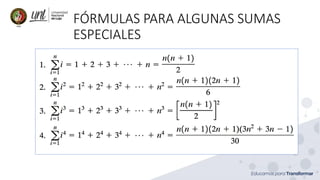
18. LA INTEGRAL DEFINIDA
Función f(x)
[a, b]
Partición P de [a, b]
0 1 2 1n na x x x x x b−=      =
1i i ix x x − = −
( )
1
n
P i i
i
R f x x
=
=  SUMA DE RIEMANN

19. LA INTEGRAL DEFINIDA
( )
1
n
P i i
i
R f x x
=
= 

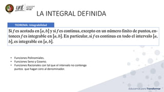
20. EJEMPLO
Evalúe la suma de Riemann para en el intervalo [-1, 2]; utilice la partición de puntos
igualmente espaciados -1 < -0.5 < 0 < 0.5 < 1 < 1.5 < 2 y tome como punto muestral al punto medio del
i-ésimo subintervalo
( ) 2
1f x x= +
ix
( )
6
1
P i i
i
R f x x
=
= 
( ) ( ) ( ) ( ) ( ) ( ) ( )0.75 0.25 0.25 0.75 1.25 1.75 0.5f f f f f f= − + − + + + +  
 ( )1.5625 1.0625 1.0625 1.5625 2.5625 4.0625 0.5= + + + + +
5.9375=

21. LA INTEGRAL DEFINIDA
( )
1
n
P i i
i
R f x x
=
= 

22. LA INTEGRAL DEFINIDA
DEFINICIÓN: Integral Definida

23. LA INTEGRAL DEFINIDA
( )
b
arriba abajoa
f x dx A A= −
( )
( ) ( )
0
,
a
a
b a
a b
f x dx
f x dx f x dx a b
=
= − 

 

24. LA INTEGRAL DEFINIDA
TEOREMA: Integrabilidad
• Funciones Polinomiales.
• Funciones Seno y Coseno.
• Funciones Racionales con tal que el intervalo no contenga
puntos que hagan cero al denominador.

25. EJEMPLO
( )
3
2
3x dx
−
+
Dividimos en intervalo [-2, 3] en n subintervalos iguales, cada uno de longitud . En cada
subintervalo utilícese como el punto de muestra.
5x n =
 1,i ix x− i ix x=
0 2x = −
1
5
2 2x x
n
= − +  = − +
2
5
2 2 2 2x x
n
 
= − +  = − +  
 
5
2 2ix i x i
n
 
= − +  = − +  
 
5
2 2 3nx n x n
n
 
= − +  = − + = 
 
( )
5
3 1i if x x i
n
 
= + = +  
 
( ) ( )
1 1
n n
i i i
i i
f x x f x x
= =
 =  
1
5 5
1
n
i
i
n n=
  
= +   
  

2
1 1
5 25
1
n n
i i
i
n n= =
= + 
5 25 1
1
2
n
n n
 
= + + 
 
25 1
5 1
2 n
 
= + + 
 

26. EJEMPLO
( )
3
2
3x dx
−
+
Dividimos en intervalo [-2, 3] en n subintervalos iguales, cada uno de longitud . En cada
subintervalo utilícese como el punto de muestra.
5x n =
 1,i ix x− i ix x=
25 1
5 1
2 n
 
= + + 
 
P es una partición regular
( ) ( )
3
2 0
1
3 lim
n
i i
P
i
x dx f x x
− →
=
+ = 
25 1
lim 5 1
2n n→
  
= + +  
  
35
2
=
( ) ( )
1 1 35
1 6 5
2 2 2
A a b h= + = + =

27. LA INTEGRAL DEFINIDA
( ) ( ) ( ) ( )1 2 1 2A R A R R A R A R=  = +
( ) ( ) ( )
c b c
a a b
f x dx f x dx f x dx= +  

28. LA INTEGRAL DEFINIDA
TEOREMA: Propiedad Aditiva para Intervalos

29. PRIMER TEOREMA FUNDAMENTAL
DEL CÁLCULO
El Cálculo es el estudio de los límites
Derivada Integral Definida
( )
( ) ( )
0
' lim
h
f x h f x
f x
h→
+ −
= ( ) ( )0
1
lim
nb
i ia P
i
f x dx f x x
→
=
= 

30. PRIMER TEOREMA FUNDAMENTAL
DEL CÁLCULO
TEOREMA: Primer Teorema Fundamental del Cálculo

31. PRIMER TEOREMA FUNDAMENTAL
DEL CÁLCULO
TEOREMA: Propiedad de Comparación

32. PRIMER TEOREMA FUNDAMENTAL
DEL CÁLCULO
TEOREMA: Propiedad de Acotamiento

33. PRIMER TEOREMA FUNDAMENTAL
DEL CÁLCULO
TEOREMA: Linealidad de la Integral Definida

34. EJEMPLO
3
1
xd
t dt
dx
 
  Encuentre
3 3
1
xd
t dt x
dx
  =
  
Determine
3
2
22
17
xd t
dt
dx t
 
 
 + 

3 3
2 2
2 22
17 17
xd t x
dt
dx t x
 
  =
 + + 

Encuentre ( ) ( )
4
2 3
tan cos ,
2 2x
d
u u du x
dx
    
  
( ) ( ) ( ) ( )
4
2 2
4
tan cos tan cos
x
x
d d
u u du u u du
dx dx
   = −
       
( ) ( ) ( ) ( )2 2
4
tan cos tan cos
xd
u u du x x
dx
 = − = −
  

35. PREGUNTAS